An Introduction to Computational Physics ppt
Bạn đang xem bản rút gọn của tài liệu. Xem và tải ngay bản đầy đủ của tài liệu tại đây (1.75 MB, 402 trang )
An Introduction to Computational Physics
Numerical simulation is now an integrated part of science and technology. Now
in its second edition, this comprehensive textbook provides an introduction to
the basic methods of computational physics, as well as an overview of recent
progress in several areas of scientific computing. The author presents many
step-by-step examples, including program listings in Java
TM
, of practical
numerical methods from modern physics and areas in which computational
physics has made significant progress in the last decade.
The first half of the book deals with basic computational tools and routines,
covering approximation and optimization of a function, differential equations,
spectral analysis, and matrix operations. Important concepts are illustrated by
relevant examples at each stage. The author also discusses more advanced
topics, such as molecular dynamics, modeling continuous systems, Monte
Carlo methods, the genetic algorithm and programming, and numerical
renormalization.
This new edition has been thoroughly revised and includes many more
examples and exercises. It can be used as a textbook for either undergraduate or
first-year graduate courses on computational physics or scientific computation.
It will also be a useful reference for anyone involved in computational research.
Tao Pang is Professor of Physics at the University of Nevada, Las Vegas.
Following his higher education at Fudan University, one of the most prestigious
institutions in China, he obtained his Ph.D. in condensed matter theory from the
University of Minnesota in 1989. He then spent two years as a Miller Research
Fellow at the University of California, Berkeley, before joining the physics
faculty at the University of Nevada, Las Vegas in the fall of 1991. He has been
Professor of Physics at UNLV since 2002. His main areas of research include
condensed matter theory and computational physics.
An Introduction to
Computational Physics
Second Edition
Tao Pang
University of Nevada, Las Vegas
cambridge university press
Cambridge, New York, Melbourne, Madrid, Cape Town, Singapore, São Paulo
Cambridge University Press
The Edinburgh Building, Cambridge cb2 2ru,UK
First published in print format
isbn-13 978-0-521-82569-6
isbn-13 978-0-521-53276-1
isbn-13 978-0-511-14046-4
© T. Pang 2006
2006
Informationonthistitle:www.cambrid
g
e.or
g
/9780521825696
This publication is in copyright. Subject to statutory exception and to the provision of
relevant collective licensing agreements, no reproduction of any part may take place
without the written permission of Cambridge University Press.
isbn-10 0-511-14046-0
isbn-10 0-521-82569-5
isbn-10 0-521-53276-0
Cambridge University Press has no responsibility for the persistence or accuracy of urls
for external or third-party internet websites referred to in this publication, and does not
guarantee that any content on such websites is, or will remain, accurate or appropriate.
Published in the United States of America by Cambridge University Press, New York
www.cambridge.org
hardback
eBook (NetLibrary)
eBook (NetLibrary)
hardback
To Yunhua, for enduring love
Contents
Preface to first edition xi
Preface xiii
Acknowledgments xv
1 Introduction 1
1.1 Computation and science 1
1.2 The emergence of modern computers 4
1.3 Computer algorithms and languages 7
Exercises 14
2 Approximation of a function 16
2.1 Interpolation 16
2.2 Least-squares approximation 24
2.3 The Millikan experiment 27
2.4 Spline approximation 30
2.5 Random-number generators 37
Exercises 44
3 Numerical calculus 49
3.1 Numerical differentiation 49
3.2 Numerical integration 56
3.3 Roots of an equation 62
3.4 Extremes of a function 66
3.5 Classical scattering 70
Exercises 76
4 Ordinary differential equations 80
4.1 Initial-value problems 81
4.2 The Euler and Picard methods 81
4.3 Predictor–corrector methods 83
4.4 The Runge–Kutta method 88
4.5 Chaotic dynamics of a driven pendulum 90
4.6 Boundary-value and eigenvalue problems 94
vii
viii Contents
4.7 The shooting method 96
4.8 Linear equations and the Sturm–Liouville problem 99
4.9 The one-dimensional Schr¨odinger equation 105
Exercises 115
5 Numerical methods for matrices 119
5.1 Matrices in physics 119
5.2 Basic matrix operations 123
5.3 Linear equation systems 125
5.4 Zeros and extremes of multivariable functions 133
5.5 Eigenvalue problems 138
5.6 The Faddeev–Leverrier method 147
5.7 Complex zeros of a polynomial 149
5.8 Electronic structures of atoms 153
5.9 The Lanczos algorithm and the many-body problem 156
5.10 Random matrices 158
Exercises 160
6 Spectral analysis 164
6.1 Fourier analysis and orthogonal functions 165
6.2 Discrete Fourier transform 166
6.3 Fast Fourier transform 169
6.4 Power spectrum of a driven pendulum 173
6.5 Fourier transform in higher dimensions 174
6.6 Wavelet analysis 175
6.7 Discrete wavelet transform 180
6.8 Special functions 187
6.9 Gaussian quadratures 191
Exercises 193
7 Partial differential equations 197
7.1 Partial differential equations in physics 197
7.2 Separation of variables 198
7.3 Discretization of the equation 204
7.4 The matrix method for difference equations 206
7.5 The relaxation method 209
7.6 Groundwater dynamics 213
7.7 Initial-value problems 216
7.8 Temperature field of a nuclear waste rod 219
Exercises 222
8 Molecular dynamics simulations 226
8.1 General behavior of a classical system 226
Contents ix
8.2 Basic methods for many-body systems 228
8.3 The Verlet algorithm 232
8.4 Structure of atomic clusters 236
8.5 The Gear predictor–corrector method 239
8.6 Constant pressure, temperature, and bond length 241
8.7 Structure and dynamics of real materials 246
8.8 Ab initio molecular dynamics 250
Exercises 254
9 Modeling continuous systems 256
9.1 Hydrodynamic equations 256
9.2 The basic finite element method 258
9.3 The Ritz variational method 262
9.4 Higher-dimensional systems 266
9.5 The finite element method for nonlinear equations 269
9.6 The particle-in-cell method 271
9.7 Hydrodynamics and magnetohydrodynamics 276
9.8 The lattice Boltzmann method 279
Exercises 282
10 Monte Carlo simulations 285
10.1 Sampling and integration 285
10.2 The Metropolis algorithm 287
10.3 Applications in statistical physics 292
10.4 Critical slowing down and block algorithms 297
10.5 Variational quantum Monte Carlo simulations 299
10.6 Green’s function Monte Carlo simulations 303
10.7 Two-dimensional electron gas 307
10.8 Path-integral Monte Carlo simulations 313
10.9 Quantum lattice models 315
Exercises 320
11 Genetic algorithm and programming 323
11.1 Basic elements of a genetic algorithm 324
11.2 The Thomson problem 332
11.3 Continuous genetic algorithm 335
11.4 Other applications 338
11.5 Genetic programming 342
Exercises 345
12 Numerical renormalization 347
12.1 The scaling concept 347
12.2 Renormalization transform 350
x Contents
12.3 Critical phenomena: the Ising model 352
12.4 Renormalization with Monte Carlo simulation 355
12.5 Crossover: the Kondo problem 357
12.6 Quantum lattice renormalization 360
12.7 Density matrix renormalization 364
Exercises 367
References 369
Index 381
Preface to first edition
The beauty of Nature is in its detail. If we are to understand different layers of sci-
entific phenomena, tedious computations are inevitable. In the last half-century,
computational approaches to many problems in science and engineering have
clearly evolved into a new branch of science, computational science. With the
increasing computing power of modern computers and the availability of new
numerical techniques, scientists in different disciplines have started to unfold
the mysteries of the so-called grand challenges, which are identified as scientific
problems that will remain significant for years to come and may require teraflop
computing power. These problems include, but are not limited to, global environ-
mental modeling, virus vaccine design, and new electronic materials simulation.
Computational physics, in my view, is the foundation of computational sci-
ence. It deals with basic computational problems in physics, which are closely
related to the equations and computational problems in other scientific and en-
gineering fields. For example, numerical schemes for Newton’s equation can be
implemented in the study of the dynamics of large molecules in chemistry and
biology; algorithms for solving the Schr¨odinger equation are necessary in the
study of electronic structures in materials science; the techniques used to solve
the diffusion equation can be applied to air pollution control problems; and nu-
merical simulations of hydrodynamic equations are needed in weather prediction
and oceanic dynamics.
Important as computational physics is, it has not yet become a standard course
in the curricula of many universities. But clearly its importance will increase
with the further development of computational science. Almost every college or
university now has some networked workstations available to students. Probably
many of them will have some closely linked parallel or distributed computing
systems in the near future. Students from many disciplines within science and
engineering now demand the basic knowledge of scientific computing, which
will certainly be important in their future careers. This book is written to fulfill
this need.
Some of the materials in this book come from my lecture notes for a com-
putational physics course I have been teaching at the University of Nevada, Las
Vegas. I usually have a combination of graduate and undergraduate students from
physics, engineering, and other majors. All of them have some access to the work-
stations or supercomputers on campus. The purpose of my lectures is to provide
xi
xii Preface to first edition
the students with some basic materials and necessary guidance so they can work
out the assigned problems and selected projects on the computers available to
them and in a programming language of their choice.
This book is made up of two parts. The first part (Chapter 1 through Chapter 6)
deals with the basics of computational physics. Enough detail is provided so that a
well-prepared upper division undergraduate student in science or engineering will
have no difficulty in following the material. The second part of the book (Chapter 7
through Chapter 12) introduces some currently used simulation techniques and
some of the newest developments in the field. The choice of subjects in the second
part is based on my judgment of the importance of the subjects in the future. This
part is specifically written for students or beginning researchers who want to know
the new directions in computational physics or plan to enter the research areas of
scientific computing. Many references are given there to help in further studies.
In order to make the course easy to digest and also to show some practical
aspects of the materials introducedin the text, I have selected quitea few exercises.
The exercises have different levels of difficulty and can be grouped into three
categories. Those in the first category are simple, short problems; a student with
little preparation can still work them out with some effort at filling in the gaps
they have in both physics and numerical analysis. The exercises in the second
category are more involved and aimed at well-prepared students. Those in the third
category are mostly selected from current research topics, which will certainly
benefit those students who are going to do research in computational science.
Programs for the examples discussed in the text are all written in standard
Fortran 77, with a few exceptions that are available on almost all Fortran compil-
ers. Some more advanced programming languages for data parallel or distributed
computing are also discussed in Chapter 12. I have tried to keep all programs in
the book structured and transparent, and I hope that anyone with knowledge of any
programming language will be able to understand the content without extra effort.
As a convention, all statements are written in upper case and all comments are
given in lower case. From my experience, this is the best way of presenting a clear
and concise Fortran program. Many sample programs in the text are explained
in sufficient detail with commentary statements. I find that the most efficient
approach to learning computational physics is to study well-prepared programs.
Related programs used in the book can be accessed via the World Wide Web at
the URL Corre-
sponding programs in C and Fortran 90 and other related materials will also be
available at this site in the future.
This book can be used as a textbook for a computational physics course.
If it is a one-semester course, my recommendation is to select materials from
Chapters 1 through 7 and Chapter 11. Some sections, such as 4.6 through 4.8,
5.6, and 7.8, are good for graduate students or beginning researchers but may
pose some challenges to most undergraduate students.
Tao Pang
Las Vegas, Nevada
Preface
Since the publication of the first edition of the book, I have received numerous
comments and suggestions on the book from all over the world and from a far
wider range of readers than anticipated. This is a firm testament of what I claimed
in the Preface to the first edition that computational physics is truly the foundation
of computational science.
The Internet, which connects all computerized parts of the world, has made it
possible to communicate with students who are striving to learn modern science in
distant places that I have never even heard of. The main drive for having a second
edition of the book is to provide a new generation of science and engineering
students with an up-to-date presentation to the subject.
In the last decade, we have witnessed steady progress in computational studies
of scientific problems. Many complex issues are now analyzed and solved on
computers. New paradigms of global-scale computing have emerged, such as the
Grid and web computing. Computers are faster and come with more functions
and capacity. There has never been a better time to study computational physics.
For this new edition, I have revised each chapter in the book thoroughly, incor-
porating many suggestions made by the readers of the first edition. There are more
examples given with more sample programs and figures to make the explanation
of the material easier to follow. More exercises are given to help students digest
the material. Each sample program has been completely rewritten to reflect what
I have learned in the last few years of teaching the subject. A lot of new material
has been added to this edition mainly in the areas in which computational physics
has made significant progress and a difference in the last decade, including one
chapter on genetic algorithm and programming. Some material in the first edition
has been removed mainly because there are more detailed books on those subjects
available or they appear to be out of date. The website for this new edition is at
/>References are cited for the sole purpose of providing more information for
further study on the relevant subjects. Therefore they may not be the most author-
itative or defining work. Most of them are given because of my familiarity with,
or my easy access to, the cited materials. I have also tried to limit the number of
references so the reader will not find them overwhelming. When I have had to
choose, I have always picked the ones that I think will benefit the readers most.
xiii
xiv Preface
Java is adopted as the instructional programming language in the book. The
source codes are made available at the website. Java, an object-oriented and
interpreted language, is the newest programming language that has made a major
impact in the last few years. The strength of Java is in its ability to work with web
browsers, its comprehensive API (application programming interface), and its
built-in security and network support. Both the source code and bytecode can run
on any computer that has Java with exactly the same result. There are many advan-
tages in Java, and its speed in scientific programming has steadily increased over
the last few years. At the moment, a carefully written Java program, combined
with static analysis, just-in-time compiling, and instruction-level optimization,
can deliver nearly the same raw speed as C or Fortran. More scientists, especially
those who are still in colleges or graduate schools, are expected to use Java as
their primary programming language. This is why Java is used as the instructional
language in this edition. Currently, many new applications in science and engi-
neering are being developed in Java worldwide to facilitate collaboration and to
reduce programming time. This book will do its part in teaching students how to
build their own programs appropriate for scientific computing. We do not know
what will be the dominant programming language for scientific computing in the
future, but we do know that scientific computing will continue playing a major
role in fundamental research, knowledge development, and emerging technology.
Acknowledgments
Most of the material presented in this book has been strongly influenced by my
research work in the last 20 years, and I am extremely grateful to the University of
Minnesota, the Miller Institute for Basic Research in Science at the University of
California, Berkeley, the National Science Foundation, the Department of Energy,
and the W. M. Keck Foundation for their generous support of my research work.
Numerous colleagues from all over the world have made contributions to this
edition while using the first edition of the book. My deepest gratitude goes to those
who have communicated with me over the years regarding the topics covered in
the book, especially those inspired young scholars who have constantly reminded
me that the effort of writing this book is worthwhile, and the students who have
taken the course from me.
xv
Chapter 1
Introduction
Computing has become a necessary means of scientific study. Even in ancient
times, the quantification of gained knowledge played an essential role in the
further development of mankind. In this chapter, we will discuss the role of
computation in advancing scientific knowledge and outline the current status of
computational science. We will only provide a quick tour of the subject here.
A more detailed discussion on the development of computational science and
computers can be found in Moreau (1984) and Nash (1990). Progress in parallel
computing and global computing is elucidated in Koniges (2000), Foster and
Kesselman (2003), and Abbas (2004).
1.1 Computation and science
Modern societies are not the only ones to rely on computation. Ancient societies
also had to deal with quantifying their knowledgeandevents. It is interesting tosee
how the ancient societies developed their knowledge of numbers and calculations
with different means and tools. There is evidence that carved bones and marked
rocks were among the early tools used for recording numbers and values and for
performing simple estimates more than 20 000 years ago.
The most commonly used number system today is the decimal system, which
was in existence in India at least 1500 years ago. It has a radix (base) of 10.
A number is represented by a string of figures, with each from the ten available
figures (0–9) occupying a different decimal level. The way a number is represented
in the decimal system is not unique. All other number systems have similar
structures, even though their radices are quite different, for example, the binary
system used on all digital computers has a radix of 2. During almost the same era
in which the Indians were using the decimal system, another number system using
dots (each worth one) and bars (each worth five) on a base of 20 was invented
by the Mayans. A symbol that looks like a closed eye was used for zero. It is
still under debate whether the Mayans used a base of 18 instead of 20 after the
first level of the hierarchy in their number formation. They applied these dots
and bars to record multiplication tables. With the availability of those tables, the
1
2 Introduction
0
1
5
20
=
15 17 255=
(a)
(b)
Fig. 1.1 The Mayan
number system: (a)
examples of using dots
and bars to represent
numbers; (b) an example
of recording
multiplication.
1
π/ k
l
k
d =
Fig. 1.2 A circle inscribed
and circumscribed by two
hexagons. The inside
polygon sets the lower
bound while the outside
polygon sets the upper
bound of the
circumference.
Mayans studied and calculated the period of lunar eclipses to a great accuracy.
An example of Mayan number system is shown in Fig. 1.1.
One of the most fascinating numbers ever calculated in human history is π,
the ratio of the circumference to the diameter of the circle. One of the methods of
evaluating π was introduced by Chinese mathematician Liu Hui, who published
his result in a book in the third century. The circle was approached and bounded
by two sets of regular polygons, one from outside and another from inside of
the circle, as shown in Fig. 1.2. By evaluating the side lengths of two 192-sided
regular polygons, Liu found that 3.1410 <π<3.1427, and later he improved
his result with a 3072-sided inscribed polygon to obtain π 3.1416. Two hun-
dred years later, Chinese mathematician and astronomer Zu Chongzhi and his son
Zu Gengzhi carried this type of calculation much further by evaluating the side
lengths of two 24 576-sided regular polygons. They concluded that 3.141 592 6 <
π<3.141 592 7, and pointed out that a good approximation was given by
1.1 Computation and science 3
π 355/113 = 3.141 592 9 This is extremely impressive considering the
limited mathematics and computing tools that existed then. Furthermore, no one
in the next 1000 years did a better job of evaluating π than the Zus.
The Zus could have done an even better job if they had had any additional help
in either mathematical knowledge or computing tools. Let us quickly demonstrate
this statement by considering a set of evaluations on polygons with a much smaller
number of sides. In general, if the side length of a regular k-sided polygon is
denoted as l
k
and the corresponding diameter is taken to be the unit of length,
then the approximation of π is given by
π
k
= kl
k
. (1.1)
The exact value of π is the limit of π
k
as k →∞. The value of π
k
obtained from
the calculations of the k-sided polygon can be formally written as
π
k
= π
∞
+
c
1
k
+
c
2
k
2
+
c
3
k
3
+···, (1.2)
where π
∞
= π and c
i
, for i = 1, 2, ,∞, are the coefficients to be determined.
The expansion in Eq. (1.2) is truncated in practice in order to obtain an approxi-
mation of π. Then the task left is to solve the equation set
n
j=1
a
ij
x
j
= b
i
, (1.3)
for i = 1, 2, , n, if the expansion in Eq. (1.2) is truncated at the (n − 1)th
order of 1/k with a
ij
= 1/k
j−1
i
, x
1
= π
∞
, x
j
= c
j−1
for j > 1, and b
i
= π
k
i
. The
approximation of π is then given by the approximate π
∞
obtained by solving the
equation set. For example, if π
8
= 3.061 467, π
16
= 3.121 445, π
32
= 3.136 548,
and π
64
= 3.140 331 are given from the regular polygons inscribing the circle, we
can truncate the expansion at the third order of 1/k and then solve the equation
set (see Exercise 1.1) to obtain π
∞
, c
1
, c
2
, and c
3
from the given π
k
. The approxi-
mation of π π
∞
is 3.141 583, which has five digits of accuracy, in comparison
with the exact value π = 3.141 592 65 The values of π
k
for k = 8, 16, 32, 64
and the extrapolation π
∞
are all plotted in Fig. 1.3. The evaluation can be further
improved if we use more π
k
or ones with higher values of k. For example, we
obtain π 3.141 592 62 if k = 32, 64, 128, 256 are used. Note that we are get-
ting the same accuracy here as the evaluation of the Zus with polygons of 24 576
sides.
In a modern society, we need to deal with a lot more computations daily.
Almost every event in science or technology requires quantification of the data in-
volved. For example, before a jet aircraft can actually be manufactured, extensive
computer simulations in different flight conditions must be performed to check
whether there is a design flaw. This is not only necessary economically, but may
help avoid loss of lives. A related use of computers is in the reconstruction of an
unexpectred flight accident. This is extremely important in preventing the same
accident from happening again. A more common example is found in the cars
4 Introduction
3.05
3.07
3.09
3.11
3.13
3.15
0.00 0.03 0.06 0.09 0.12 0.15
π
k
1/k
×
×
×
×
×
Fig. 1.3 The values of π
k
,
with k = 8, 16, 32, and 64,
plotted together with the
extrapolated π
∞
.
that we drive, which each have a computer that takes care of the brakes, steering
control, and other critical components. Almost any electronic device that we use
today is probably powered by a computer, for example, a digital thermometer,
a DVD (digital video disc) player, a pacemaker, a digital clock, or a microwave
oven. The list can go on and on. It is fair to say that sophisticated computations
delivered by computers every moment have become part of our lives, permanently.
1.2 The emergence of modern computers
The advantage of having a reliable, robust calculating device was realized a long
time ago. The early abacus, which was used for counting, was in existence with
the Babylonians 4000 years ago. The Chinese abacus, which appeared at least
3000 years ago, was perhaps the first comprehensive calculating device that was
actually used in performing addition, subtraction, multiplication, and division
and was employed for several thousand years. A traditional Chinese abacus is
made of a rectangular wooden frame and a bar going through the upper middle
of the frame horizontally. See Fig. 1.4. There are thirteen evenly spaced vertical
rods, each representing one decimal level. More rods were added to later versions.
On each rod, there are seven beads that can be slid up and down with five of them
held below the middle bar and two above. Zero on each rod is represented by the
beads below the middle bar at the very bottom and the beads above at the very
top. The numbers one to four are repsented by sliding one–four beads below the
middle bar up and five is given be sliding one bead above down. The numbers six
to nine are represented by one bead above the middle bar slid down and one–four
beads below slid up. The first and last beads on each rod are never used or are
only used cosmetically during a calculation. The Japanese abacus, which was
modeled on the Chinese abacus, in fact has twenty-one rods, with only five beads
1.2 The emergence of modern computers 5
Fig. 1.4 A sketch of a
Chinese abacus with
the number 15 963.82
shown.
on each rod, one above and four below the middle bar. Dots are marked on the
middle bar for the decimal point and for every four orders (ten thousands) of
digits. The abacus had to be replaced by the slide rule or numerical tables when
a calcualtion went beyond the four basic operations even though later versions
of the Chinese abacus could also be used to evaluate square roots and cubic
roots.
The slide rule, which is considered to be the next major advance in calculat-
ing devices, was introduced by the Englishmen Edmund Gunter and Reverend
William Oughtred in the mid-seventeenth century based on the logarithmic table
published by Scottish mathematician John Napier in a book in the early seven-
teenth century. Over the next several hundred years, the slide rule was improved
and used worldwide to deliver the impressive computations needed, especially
during the Industrial Revolution. At about the same time as the introduction of the
slide rule, Frenchman Blaise Pascal invented the mechanical calculating machine
with gears of different sizes. The mechanical calculating machine was enhanced
and applied extensively in heavy-duty computing tasks before digital computers
came into existence.
The concept of an all-purpose, automatic, and programmable computing ma-
chine was introduced by British mathematician and astronomer Charles Babbage
in the early nineteenth century. After building part of a mechanical calculating
machine that he called a difference engine, Babbage proposed constructing a
computing machine, called an analytical engine, which could be programmed to
perform any type of computation. Unfortunately, the technology at the time was
not advanced enough to provide Babbage with the necessary machinery to realize
his dream. In the late nineteenth century, Spanish engineer Leonardo Torres y
Quevedo showed that it might be possible to construct the machine conceived
earlier by Babbage using the electromechanical technology that had just been
developed. However, he could not actually build the whole machine either, due
to lack of funds. American engineer and inventor Herman Hollerith built the
very first electromechanical counting machine, which was commisioned by the
US federal government for sorting the population in the 1890 American census.
Hollerith used the profit obtained from selling this machine to set up a com-
pany, the Tabulating Machine Company, the predecessor of IBM (International
6 Introduction
Business Machines Corporation). These developments continued in the early
twentieth century. In the 1930s, scientists and engineers at IBM built the first
difference tabulator, while researchers at Bell Laboratories built the first relay
calculator. These were among the very first electromechanical calculators built
during that time.
The real beginning of the computer era came with the advent of electronic
digital computers. John Vincent Atanasoff, a theoretical physicist at the Iowa
State University at Ames, invented the electronic digital computer between 1937
and 1939. The history regarding Atanasoff’s accomplishment is described in
Mackintosh (1987), Burks and Burks (1988), and Mollenhoff (1988). Atanasoff
introduced vacuum tubes (instead of the electromechanical devices used ear-
lier by other people) as basic elements, a separated memory unit, and a scheme
to keep the memory updated in his computer. With the assistance of Clifford
E. Berry, a graduate assistant, Atanasoff built the very first electronic computer
in 1939. Most computer history books have cited ENIAC (Electronic Numeri-
cal Integrator and Computer), built by John W. Mauchly and J. Presper Eckert
with their colleagues at the Moore School of the University of Pennsylvania in
1945, as the first electronic computer. ENIAC, with a total mass of more than
30 tons, consisited of 18 000 vacuum tubes, 15 000 relays, and several hundred
thousand resistors, capacitors, and inductors. It could complete about 5000 ad-
ditions or 400 multiplications in one second. Some very impressive scientific
computations were performed on ENIAC, including the study of nuclear fis-
sion with the liquid drop model by Metropolis and Frankel (1947). In the early
1950s, scientists at Los Alamos built another electronic digital computer, called
MANIAC I (Mathematical Analyzer, Numerator, Integrator, and Computer),
which was very similar to ENIAC. Many important numerical studies, includ-
ing Monte Carlo simulation of classical liquids (Metropolis et al., 1953), were
completed on MANIAC I.
All these research-intensive activities accomplished in the 1950s showed that
computation was no longer just a supporting tool for scientific research but rather
an actual means of probing scientific problems and predicting new scientific
phenomena. A new branch of science, computational science, was born. Since
then, the field of scientific computing has developed and grown rapidly.
The computational power of new computers has been increasing exponentially.
To be specific, the computing power of a single computer unit has doubled almost
every 2 years in the last 50 years. This growth followed the observation of Gordon
Moore, co-founder of Intel, that information stored on a given amount of silicon
surface had doubled and would continue to do so in about every 2 years since the
introduction of the silicon technology (nicknamed Moore’s law). Computers with
transistors replaced those with vacuum tubes in the late 1950s and early 1960s,
and computers with very-large-scale integrated circuits were built in the 1970s.
Microprocessors and vector processors were built in the mid-1970s to set the
1.3 Computer algorithms and languages 7
stage for personal computing and supercomputing. In the 1980s, microprocessor-
based personal computers and workstations appeared. Now they have penetrated
all aspects of our lives, as well as all scientific disciplines, because of their afford-
ability and low maintenance cost. With technological breakthroughs in the RISC
(Reduced Instruction Set Computer) architecture, cache memory, and multiple
instruction units, the capacity of each microprocessor is now larger than that of a
supercomputer 10 years ago. In the last few years, these fast microprocessors have
been combined to form parallel or distributed computers, which can easily deliver
a computing power of a few tens of gigaflops (10
9
floating-point operations per
second). New computing paradigms such as the Grid were introduced to utilize
computing resources on a global scale via the Internet (Foster and Kesselman,
2003; Abbas, 2004).
Teraflop (10
12
floating-point operations per second) computers are now emerg-
ing. For example, Q, a newly installed computer at the Los Alamos National
Laboratory, has a capacity of 30 teraflops. With the availability of teraflop com-
puters, scientists can start unfolding the mysteries of the grand challenges, such as
the dynamics of the global environment; the mechanism of DNA (deoxyribonu-
cleic acid) sequencing; computer design of drugs to cope with deadly viruses;
and computer simulation of future electronic materials, structures, and devices.
Even though there are certain problems that computers cannot solve, as pointed
out by Harel (2000), and hardware and software failures can be fatal, the human
minds behind computers are nevertheless unlimited. Computers will never replace
human beings in this regard and the quest for a better understanding of Nature
will go on no matter how difficult the journey is. Computers will certainly help
to make that journey more colorful and pleasant.
1.3 Computer algorithms and languages
Before we can use a computer to solve a specific problem, we must instruct the
computer to follow certain procedures and to carry out the desired computational
task. The process involves two steps. First, we need to transform the problem,
typically in the form of an equation, into a set of logical steps that a computer
can follow; second, we need to inform the computer to complete these logical
steps.
Computer algorithms
The complete set of the logical steps for a specific computational problem is called
a computer or numerical algorithm. Some popular numerical algorithms can be
traced back over a 100 years. For example, Carl Friedrich Gauss (1866) pub-
lished an article on the FFT (fast Fourier transform) algorithm (Goldstine, 1977,
8 Introduction
pp. 249–53). Of course, Gauss could not have envisioned having his algorithm
realized on a computer.
Let us use a very simple and familiar example in physics to illustrate how a
typical numerical algorithm is constructed. Assume that a particle of mass m is
confined to move along the x axis under a force f (x). If we describe its motion
with Newton’s equation, we have
f = ma = m
dv
dt
, (1.4)
where a and v are the acceleration and velocity of the particle, respectively, and
t is the time. If we divide the time into small, equal intervals τ = t
i+1
− t
i
,we
know from elementary physics that the velocity at time t
i
is approximately given
by the average velocity in the time interval [t
i
, t
i+1
],
v
i
x
i+1
− x
i
t
i+1
− t
i
=
x
i+1
− x
i
τ
; (1.5)
the corresponding acceleration is approximately given by the average acceleration
in the same time interval,
a
i
v
i+1
− v
i
t
i+1
− t
i
=
v
i+1
− v
i
τ
, (1.6)
as long as τ is small enough. The simplest algorithm for finding the position and
velocity of the particle at time t
i+1
from the corresponding quantities at time t
i
is obtained after combining Eqs. (1.4), (1.5), and (1.6), and we have
x
i+1
= x
i
+ τv
i
, (1.7)
v
i+1
= v
i
+
τ
m
f
i
, (1.8)
where f
i
= f (x
i
). If the initial position and velocity of the particle are given and
the corresponding quantities at some later time are sought (the initial-value prob-
lem), we can obtain them recursively from the algorithm given in Eqs. (1.7) and
(1.8). This algorithm is commonly known as the Euler method for the initial-value
problem. This simple example illustrates how most algorithms are constructed.
First, physical equations are transformed into discrete forms, namely, difference
equations. Then the desired physical quantities or solutions of the equations at
different variable points are given in a recursive manner with the quantities at a
later point expressed in terms of the quantities from earlier points. In the above
example, the position and velocity of the particle at t
i+1
are given by the position
and velocity at t
i
, provided that the force at any position is explicitly given by a
function of the position. Note that the above way of constructing an algorithm is
not limited to one-dimensional or single-particle problems. In fact, we can im-
mediately generalize this algorithm to two-dimensional and three-dimensional
problems, or to the problems involving more than one particle, such as the