PRACTICAL APPLICATIONS AND SOLUTIONS USING LABVIEW™ SOFTWARE ppsx

PRACTICAL APPLICATIONS
AND SOLUTIONS USING
LABVIEW™ SOFTWARE

Edited by Silviu Folea











Practical Applications and Solutions Using LabVIEW™ Software
Edited by Silviu Folea


Published by InTech
Janeza Trdine 9, 51000 Rijeka, Croatia

Copyright © 2011 InTech
All chapters are Open Access articles distributed under the Creative Commons
Non Commercial Share Alike Attribution 3.0 license, which permits to copy,
distribute, transmit, and adapt the work in any medium, so long as the original
work is properly cited. After this work has been published by InTech, authors
have the right to republish it, in whole or part, in any publication of which they
are the author, and to make other personal use of the work. Any republication,
referencing or personal use of the work must explicitly identify the original source.

Statements and opinions expressed in the chapters are these of the individual contributors
and not necessarily those of the editors or publisher. No responsibility is accepted
for the accuracy of information contained in the published articles. The publisher
assumes no responsibility for any damage or injury to persons or property arising out
of the use of any materials, instructions, methods or ideas contained in the book.

Publishing Process Manager Iva Lipovic
Technical Editor Teodora Smiljanic
Cover Designer Jan Hyrat
Image Copyright Sofia, 2010. Used under license from Shutterstock.com

LabVIEW™ is a trademark of National Instruments. This publication is independent of
National Instruments, which is not affiliated with the publisher or the author, and does
not authorize, sponsor, endorse or otherwise approve this publication.

First published July, 2011
Printed in Croatia

A free online edition of this book is available at www.intechopen.com
Additional hard copies can be obtained from

Practical Applications and Solutions Using LabVIEW™ Software, Edited by Silviu Folea
p. cm.
ISBN 978-953-307-650-8

free online editions of InTech
Books and Journals can be found at
www.intechopen.com

Contents

Preface IX
Part 1 Virtual Instruments 1
Chapter 1 Virtual Instrument for Online Electrical
Capacitance Tomography 3
Zhaoyan Fan, Robert X. Gao and Jinjiang Wang
Chapter 2 Low-Field NMR/MRI Systems Using LabVIEW
and Advanced Data-Acquisition Techniques 17
Aktham Asfour
Chapter 3 DH V 2.0, A Pocket PC Software to Evaluate Drip
Irrigation Lateral Diameters Fed from the Extreme with
on-line Emitters in Slope Surfaces 41
José Miguel Molina-Martínez, Manuel Jiménez-Buendía and
Antonio Ruiz-Canales
Chapter 4 Application of Virtual Instrumentation
in Nuclear Physics Experiments 57
Jiri Pechousek
Part 2 Hardware in the Loop Simulation 81
Chapter 5 Real-Time Rapid Embedded Power System
Control Prototyping Simulation
Test-Bed Using LabVIEW and RTDS 83
Karen Butler-Purry and Hung-Ming Chou
Chapter 6 The Development of a Hardware-in-the-Loop Simulation

System for Unmanned Aerial Vehicle Autopilot Design
Using LabVIEW 109
Yun-Ping Sun
Chapter 7 Equipment Based on the Hardware in the Loop (HIL) Concept
to Test Automation Equipment Using Plant Simulation 133
Eduardo Moreira, Rodrigo Pantoni and Dennis Brandão
VI Contents

Part 3 eHealth 153
Chapter 8 Sophisticated Biomedical Tissue Measurement Using Image
Analysis and Virtual Instrumentation 155
Libor Hargaš, Dušan Koniar and Stanislav Štofan
Chapter 9 Instrument Design, Measurement and Analysis of
Cardiovascular Dynamics Based on LabVIEW 181
Wei He, Hanguang Xiao, Songnong Li and Delmo Correia
Chapter 10 ECG Ambulatory System for Long Term Monitoring
of Heart Rate Dynamics 201
Agustín Márquez-Espinoza, José G. Mercado-Rojas,
Gabriel Vega-Martínez and Carlos Alvarado-Serrano
Part 4 Test and Fault Diagnosis 227
Chapter 11 Acoustical Measurement and Fan Fault Diagnosis
System Based on LabVIEW 229
Guangzhong Cao
Chapter 12 Condition Monitoring of Zinc Oxide Surge Arresters 253
Novizon, Zulkurnain Abdul-Malek, Nouruddeen Bashir and Aulia
Part 5 Practical Applications 271
Chapter 13 Remote Instrumentation Laboratory
for Digital Signal Processors Training 273
Sergio Gallardo, Federico J. Barrero and Sergio L. Toral
Chapter 14 Digital Image Processing Using LabView 297

Rubén Posada-Gómez, Oscar Osvaldo Sandoval-González,
Albino Martínez Sibaja, Otniel Portillo-Rodríguez
and Giner Alor-Hernández
Chapter 15 Remote SMS Instrumentation Supervision
and Control Using LabVIEW 317
Rafael C. Figueiredo, Antonio M. O. Ribeiro,
Rangel Arthur and Evandro Conforti
Chapter 16 Lightning Location and Mapping System Using Time
Difference of Arrival (TDoA) Technique 343
Zulkurnain Abdul-Malek, Aulia, Nouruddeen Bashir and Novizon
Chapter 17 Computer-Based Control for Chemical Systems Using
LabVIEW
®
in Conjunction with MATLAB
®
363
Syamsul Rizal Abd Shukor,
Reza Barzin and Abdul Latif Ahmad
Contents VII

Chapter 18 Dynamic Wi-Fi Reconfigurable FPGA Based Platform
for Intelligent Traffic Systems 377
Mihai Hulea, George Dan Moiş and Silviu Folea
Part 6 Programming Techniques 397
Chapter 19 Extending LabVIEW Aptitude for Distributed Controls
and Data Acquisition 399
Luciano Catani
Chapter 20 Graphical Programming Techniques
for Effective, Fast and Responsive Execut 421
Marko Jankovec

Chapter 21 The Importance of a Deep Knowledge of LabVIEW
Environment and Techniques in Order to Develop
Effective Applications 437
Riccardo de Asmundis

Preface

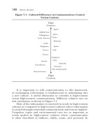
The book consists of 21 chapters which present applications implemented using the
LabVIEW environment, belonging to several distinct fields such as engineering,
chemistry, physics, fault diagnosis and medicine. In the context of the applications
presented in this book, LabVIEW offers major advantages especially due to some
characteristic features. It is a graphical programming language which utilizes
interconnected icons (functions, structures connected by wires), resembling a
flowchart and being more intuitive. Taking into account different objectives, LabVIEW
can be considered an equivalent of an alternative to the classic programming
languages. It is important to mention that the implementation time for a software
application is reduced as compared to the time needed for implementing it by using
other environments.
The built-in libraries and the virtual instruments examples (based on VIs), as well as
the software drivers for almost all the existing data acquisition systems make the
support and the use of devices produced by more than fifty companies, including
industrial instruments, oscilloscopes, multimeters and signal generators possible in
LabVIEW.
The LabVIEW platform is portable, being able to run on multiple devices and
operating systems. Programming in LabVIEW involves the creation of the graphical
code (G) on a PC, where it is afterwards compiled. Tools specific to different targets
such as industrial computers with real time operating systems (PXI), programmable
automation controllers (Compact RIO), PDAs, microcontrollers or field-programmable
gate arrays (FPGAs) are used and after that the compiled code is downloaded to the
target.
Chapter 1 presents a virtual instrument for image capture and display associated with
the electrical capacitance tomography (ECT), a noninvasive measurement method for
visualizing temporal and spatial distributions of materials within an enclosed vessel.
According to the hardware circuitry configuration and the combination of electrodes

for the ECT, the VI is implemented using seven major functional modules: switching
control, data sampling, data normalization, permittivity calculation, mesh generation,
image generation, and image display.
X Preface

Chapter 2 describes a LabVIEW based NMR spectrometer (Nuclear Magnetic
Resonance) working at low field. This spectrometer allows the detection of the NMR
signals of both 1H and
129
Xe at 4.5 mT. The aim of this chapter is to present the
advances accomplished by the author in the development of low-field NMR systems.
The flexibility of the system allows its use for a palette of NMR applications without
(or with minor) hardware and software modification.
Chapter 3 introduces a new version of drip irrigation design software (DH V 2.0) for
usage with mobile devices like Smartphones or pocket PCs. It uses LabVIEW PDA as
the programming language. The software allows the users of drip irrigation systems to
evaluate their sensibility to changing conditions (water needs, emitters, spacing, slope,
etc.) for all the diameters of commercial polythene drip lines.
Chapter 4 presents a new method for the design of computer-based measurement
systems that can be seen in the use of up-to-date measurement, control and testing
systems based on reliable devices. The measurement systems built with the help of the
LabVIEW modular instrumentation offer a popular approach to nuclear spectrometers
construction. By replacing the former single-purpose system, units with universal data
acquisition modules, a lower-cost solution that is reliable, fast, and takes high-quality
measurements, is achieved.
Chapter 5 describes a real-time rapid embedded control prototyping simulation and a
simple power system case study implementation. The detailed implementation of an
overcurrent relay for controller-in-the-loop simulation is described, including the
setting and programming of a real-time digital simulator and the programming in
CompactRIO, which includes the FPGA and the real-time processor by using

LabVIEW. A synchronization technique which allows the readers to make the
correction decision on the method to be used based on the application and its
requirements is proposed and also discussed.
Chapter 6 presents a continuing research on the design and verification of an autopilot
system for an unmanned aerial vehicle (UAV) through hardware-in-the-loop (HIL)
simulations. The software development environment used for HIL simulations is
LabVIEW. Different control methods for developing the UAV autopilot system design
are applied and the comparison between the results obtained from HIL simulations is
presented in this chapter.
Chapter 7 proposes a HIL-based system, where a Foundation Fieldbus control system
manages the simulation of a generic plant in an industrial process. The simulation
software is executed on a PC, and it has a didactic purpose for engineering students
learning to control a process similar to the real one. The plant is simulated on a
computer, implemented in LabVIEW and represents a part of the fieldbus network
simulator FBSIMU.
Chapter 8 presents a solution for measuring object beating frequency from a video
sequence using tools of image analysis and spectral analysis. It simplifies the methods
Preface XI

used in present times and reduces the usage of the hardware devices. Using the
LabVIEW environment, the authors created a fully automated application with
interactive inputting of some parameters. Several algorithms were tested on phantoms
with defined frequency. The designed hardware data acquisition system can be used
with or without microscope in applications where the placement of kinematic
parameters sensors is not possible. Intelligent regulation of condenser illumination
through image feature extraction and histogram analysis enables the fully automated
approach to video sequence acquisition.
Chapter 9 describes the design of a product developed by the authors using LabVIEW.
It is named YF/XGYD atherosclerosis detection system. The hardware and software
designs of the arterial elasticity measurement system are detailed. The system can

diagnose the condition of arterial elasticity and the degree of arteriosclerosis.
Chapter 10 proposes a prototype of an ECG telemetry system that fulfills the
requirements of real-time transmission of long term records, low power consumption
and low cost. The software for implementing the acquisition, display and storage of
the 4 signals (3 for ECG leads and one for battery voltage), the detection of the ECG R
wave peak and for processing the R-R intervals based on LabVIEW was developed for
the study of heart rate dynamics.
Chapter 11 presents an intelligent fault diagnosis system, where the noise produced by
a fan is considered to be the diagnosis signal, a non-connect measurement method is
adopted and a non-linear mapping from feature space to defective space using the
wavelet neural network is performed. Modular programming was adopted for the
development of this system, so it is easier to extend and change the characteristics of
the network fault and structure parameters.
Chapter 12 describes a new shifted current method technique for determining ZnO
ageing that was successfully implemented in LabVIEW software and was proven
useful for on-site measurement purposes. The developed program provides
convenience in the system management and a user-friendly interface.
Chapter 13 presents a remote measurement laboratory based on LabVIEW that has
been designed and implemented. It provides the users with access to remote
measurement instrumentation and a DSP embedded board, delivering different
activities related to digital signal processing and measurement experiments. End-user
Quality of Service has been measured and expressed in terms of satisfaction or
technical terms.
Chapter 14 describes different digital image processing algorithms using LabVIEW.
The chapter presents the image acquisition task and some of the most common
operations that can be locally or globally applied. The statistical information generated
by the image in a histogram is also discussed. A pattern recognition section shows
how to use an image into a computer vision application through an example of object
XII Preface

detection. All these, along with the use of other functionalities of LabVIEW lead to the
conclusion that this software is an excellent platform for developing robotic projects as
well as vision and image processing applications.
Chapter 15 presents the feasibility of a flexible and low cost monitoring and control
solution using SMS, which can be easily applied and adapted to various applications.
The developed system was applied to a RF signal procedure measurement for saving
time and staff in this process. The tool development and its use in a specific
application outline the LabVIEW versatility.
Chapter 16 introduces a new method for determining the coordinates of any cloud-to-
ground lightning strike within a certain localized region. The system is suitable for
determining distributions of lightning strikes for a small area by measuring the
induced voltages due to lightning strikes in the vicinity of an existing telephone air
line.
Chapter 17 presents a solution using two software development platforms, MATLAB
and LabVIEW, for the proper control of a microreactor-based miniaturized intensified
system. The use of the SIMULINK Interface Toolkit is presented. It enables the user to
transfer measurement data from LabVIEW to the embedded control module in
SIMULINK and also to apply the controller output to the system via LabVIEW.
Chapter 18 proposes a software and hardware platform based on a FPGA board to
which a Wi-Fi communication device has been added in order to make remote
wireless reconfiguration possible. This feature introduces a high level of flexibility
allowing the development of applications which can quickly adapt to changes in
environmental conditions and which can react to unexpected events with high speed.
The capabilities introduced by wireless technology and reconfigurable systems are
important in road traffic control systems, which are characterized by continuous
parameter variation and unexpected event and incident occurrence.
Chapter 19 presents the development of a communication framework for distributed
control and data acquisition systems, optimized for its application to LabVIEW
distributed control, but also open and compatible with other programming languages,
being based on standard communication protocols and standard data serialization

methods.
Chapter 20 describes some general rules illustrated by examples taken from real life
applications for beginner and advanced developers. The content of this chapter
represents graphical programming techniques for better Virtual Instruments (VI)
performance and rules for a better organization of the LabVIEW code.
Chapter 21 presents a collection of considerations and suggestions, some personal and
others from LabVIEW manuals, in the direction of improving the awareness
concerning what minimum knowledge is necessary for a developer in order to be able
to develop rational, well organized and effective applications.
Preface XIII

I wish to acknowledge the efforts of all the scientists who contributed to editing this
book and to express my appreciation to the InTech team.
I’d like to dedicate this book to Dr. James Truchard, National Instruments president
and CEO, who invented NI LabVIEW graphical development software together with
Jeff Kodosky.

Silviu FOLEA
Technical University of Cluj-Napoca
Department of Automation
Romania


Part 1
Virtual Instruments

1
Virtual Instrument for Online Electrical
Capacitance Tomography
Zhaoyan Fan, Robert X. Gao* and Jinjiang Wang
Department of Mechanical Engineering, University of Connecticut,
USA
1. Introduction
Electrical capacitance tomography (ECT) is a technique invented in the 1980’s to determine
material distribution in the interior of an enclosed environment by means of external
capacitance measurements (Huang et al., 1989a, 1992b). In a typical ECT system, 8 to 16
electrodes (Yang, 2010) are symmetrically mounted inside or outside a cylindrical container,
as illustrated in Figure 1. During the period of a scanning frame, an excitation signal is
applied to one of the electrodes and the remaining electrodes are acting as detector
electrodes. Subsequently, the voltage potential at each of the detector electrodes is
measured, one at a time, by the measurement electronics to determine the inter-electrode
capacitance. Changes in these measured capacitance values indicate the variation of material
distribution within the container, e.g. air bubbles translating within an oil flow. An image of
permittivity distribution directly representing the materials distribution can be retrieved
from the capacitance data through a back-projection algorithm (Isaksen, 1996).While image

resolution associated with the ECT technique is lower than other tomographic techniques
such as CT or optical imaging, it is advantageous in terms of its non-intrusive nature,
portability, robustness, and no exposure to radiation hazard.


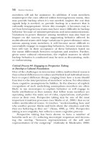
Fig. 1. Illustration of major components in an ECT system
As shown in Fig.1, an ECT system generally consists of three major components: 1) An
excitation and measurement circuitry that drives the sensors and conditions the received
signals; 2) A computer-based data acquisition (DAQ) and coordination system, to provide
control logic for the sequential excitations of the electrodes and reconstruct tomographic

Practical Applications and Solutions Using LabVIEW™ Software

4
images of the materials; as well as 3) electrodes mounted on the outer (for non-metallic
containers) or inner surface of the container.
According to the type of excitation signals being used, ECT can be divided into two
categories: AC-based (sine-wave excitation) and charge-discharge-based (square-wave
excitation). The former is advantageous in terms of measurement stability and accuracy,
whereas the latter has lower circuit complexity (Huang et al., 1992). In recent years, studies
have been conducted on sensing principle and circuit optimization to enhance the
performances of ECT. For AC-based method, a multiple excitation scheme (Fan & Gao, 2011)
has been designed and tested to increase the frame rate for higher time resolution in
monitoring fast changing dynamics inside the container. The grouping method (Olmos et
al., 2008) is another technique investigated to increase the magnitude of the received signals
by combining two or more electrodes into one segment. ECT has also been applied to
generate 3-D material distribution by mounting electrodes in multiple layers along the axis
of the cylindrical container and detecting the cross-layer capacitance values (Marashdeh &
Teixeira, 2004; Warsito et al., 2007). These efforts have expanded the scope of application of
ECT, into such fields as measurement of multi-phase flows (gas-liquid and gas-solids, etc.)

in pipelines, detection of leakage from buried water pipes, flow pattern identification
(Reinecke & Mewes, 1996; Xie et al, 2006), etc. This chapter aims to introduce the realization
of a computer-based DAQ and coordination system for ECT through Virtual
Instrumentation (VI). Discussion will focus on the AC-based method, using single excitation
and single detection channel, in which most of the basic functions required for various ECT
techniques are included. The presentation provides design guidelines and recommendations
for researchers to build ECT systems for specific applications.
2. VI design
According to the functions required for data acquisition, data processing, and circuit
control, the VI is divided into seven major subVI’s:
1. Switching control
2. Data sampling
3. Data calibration
4. Permittivity calculation
5. Mesh generation
6. Image generation
7. Image display
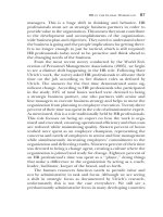
During a scanning frame, as shown in Figure 2, the Switching Control subVI divides the
process into individual measurement steps according to the total number of capacitance
values formed by all the electrodes. Connections of each electrode as well as the 8-1
multiplexer (MUX) in the measurement circuitry are controlled by the digital I/O (DIO)
ports, such that the capacitance formed by each pair of electrodes is measured in each
measurement step. After being processed by a pre-amplifier and lock-in amplifier, the
voltage signal proportional to the capacitance value is sampled by the Data Sampling
subVI. When all the capacitance values for a complete frame are sampled, they are
normalized in the Data Normalization subVI and re-sorted into the form of matrix. The
data is combined with the sensitivity matrix by the Permittivity Calculation subVI, and
finally converted into an image representing the material permittivity distribution via the
Mesh Generation, Image Generation, and Image Display subVI’s. By looping the whole

Virtual Instrument for Online Electrical Capacitance Tomography

5
process frame by frame, the VI controls the measurement circuit and samples the signal
continuously to display the dynamics of the monitored process.


Fig. 2. A detailed view of an AC-based ECT system
2.1 Switching control
The basic procedure of AC-Based capacitance measurement is to apply a sinusoidal
voltage signal to a pair of electrodes and measure the output current/voltage, from which
the impedance or capacitance can be derived (Yang, 1996). Assuming there are N
electrodes in the sensor being numbered from one to N, they are excited with the
sinusoidal wave, one at a time. When one electrode is excited, other electrodes are kept at
ground potential and act as detector electrodes. Physically, the function is realized by
controlling the SPDT (Single-Pole-Double-Throw) switch and the analog MUX as shown
in Figure 1. The common port of each SPDT switch is connected with one of the electrodes
to enable switching between the non-inverting input of a pre-amplifier (detection mode)
and the excitation source (excitation mode). In the detection mode, the output voltage
amplitude of the pre-amplifier, V
ij
, is a function of the measured inter-electrode
capacitance (Huang et al., 1992)
,
expressed as:

2
21
eij f
i

j
e
ef f
jfCR
VV
jfCR
π
π
=−
+
(1)
where C
ij
is the inter-electrode capacitance between electrodes i and j (1≤ i, j ≤ N; i ≠ j).
V
e
and f
e
are the voltage amplitude and frequency of the sine wave from the excitation
source, R
f
and C
f
are the feedback resistance and capacitance of the pre-amplifier circuit.
When the feedback resistance is chosen to satisfy the relationship |j2πf
e
C
f
R
f

|>>1, e.g.
f
e
= 700 kHz, C
f
= 50 pF, and R
f
=100 MΩ, the voltage amplitude V
ij
is approximately
proportional to C
ij
. The simplified relationship can be expressed as:

Practical Applications and Solutions Using LabVIEW™ Software

6

ij
ij e
f
C
VV
C
=−
(2)
Through the lock-in amplifier, the output sine wave from pre-amplifier is mixed with the
original excitation signal and then processed by a low pass filter. Thus a measurable DC
voltage equal to the value of
V

ij
is available from the output of the lock-in amplifier during
each individual measurement step.
The measurement protocol in the sensing electronics first measures the inter-electrode
capacitance between electrodes one and two, then between one and three, and up to one and
N. Then, the capacitances between electrodes two and three, and up to two and N are
measured. For each scanning frame, the measurements continue until all the inter-electrode
capacitances are measured and the capacitances can be represented in a matrix, which is
symmetric with respect to the diagonal. Due to
C
ij
= C
ji
, the minimum required capacitance
can be expressed as (Alme & Mylvaganam, 2007):

12
13 23
1, 1 2, 1 2, 1
1, 2, 2, 1,


NN NN
NN NNNN
C
CC
C
CC C
CC C C
−− −−

−−
⎡
⎤
⎢
⎥
⎢
⎥
⎢
⎥
=
⎢
⎥
⎢
⎥
⎢
⎥
⎣
⎦
##
(3)
With
N electrodes, this gives a total number of M independent capacitance measurements,
where
M can be expressed as (Williams & Beck, 1995):

(1)
2
NN
M
−

=
(4)
For an 8-electrode arrangement, Equation (4) gives 28 capacitance values or a total of 28
measurement steps required for each frame. Given that the SPDT switch and the 8-1 MUX
is controlled by one (log
2
2) and three (log
2
8) digital ports, respectively, a total of 8x1+3=11
digital ports are required to directly control the hardware. These digital ports can be
either connected with the DIOs on the DAQ card directly, or through a decoder to reduce
the control complexity as shown in Figure 2. The decoder translates the 5-bit digital
number sent from the DIO into the 11-bit control codes to control the switches and MUX.
Thus, the
Switching Control subVI determines electrodes for excitation and detection in
each step by sending a sequence number from 1 to 28 to the hardware decoder. Each of
the sequence number corresponds to a specific inter-electrode configuration
C
ij
, as shown
in Table 1.

Case # 0 1 2 3 … 5 6 … 9 10 … 14 15 … 20 21 … 27
C
ij

C
12
C
13

C
23
C
14
… C
34
C
15
…
C
45
C
16
…
C
56
C
17
…
C
67
C
18


C
78

DT 1 1 2 1 … 3 1 … 4 1 … 5 1 … 6 1 … 7
EX 2 3 3 4 … 4 5 … 5 6 … 6 7 … 7 8 … 8

Table 1. Sequence of the inter-electrode capacitance measurement during a frame (EX:
excitation electrode, DT: detection electrode)

Virtual Instrument for Online Electrical Capacitance Tomography

7
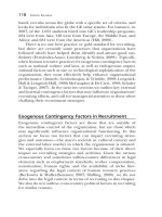
Figure 3 shows the design of the Switching Control subVI. A case structure was created to
generate the 28 sequence numbers in a binary form from 0x0001 (decimal 1, in case #0) to
1x1100 (decimal 28, in case #27). Within a
timed loop structure, the loop counter is used as
a
measurement step indicator to successively increase the control bit of the case structure till all
the 28 capacitance values are measured. The time period of each measurement step is
controlled by the loop timer,
dt, with a unit of millisecond as shown in Figure 3. The value of
dt finally determines the time resolution or the frame rate of ECT imaging. For example,
when the value of
dt is set to 4 [ms], the total time period for a frame is 28 x 4 = 112 ms,
corresponding to a maximum frame rate of 8.9 frames per second. The minimum resolution
of timer setting is constrained to one millisecond in the general LabVIEW system. Such a
limitation is shortened to microsecond level by applying the LabVIEW Real-Time module,
to further increase the frame rate of ECT at the cost of DAQ hardware upgrading (National
Instruments, 2001).


Fig. 3. Design of the Switching Control subVI within a timed loop
2.2 Data Sampling (ECT_Sampling.vi)
The Data Sampling subVI runs sequentially after the Switching Control subVI to read the
voltage
V

ij
from lock-in amplifier in each measurement step. A detailed view of the subVI
design is shown in Figure 4. To reduce the effect of noise from hardware components and
DAQ card, the DC voltage
V
ij
in each measurement step is sampled 50 times at a sampling
rate of 512 kSamples/sec. The results are averaged through a
MEAN subVI. The capacitance
value is calculated from
V
ij
with the known feedback capacitance, C
f
, and excitation signal
voltage amplitude,
V
e
. The relationship is expressed as:

ij
i
jf
e
V
CC
V
=−
(5)

Practical Applications and Solutions Using LabVIEW™ Software

8

Fig. 4. Design of Data Sampling subVI
A 28x1 capacitance array is created as Table 1 to store all the calculated capacitance values
for a scanning frame. As soon as one measurement step finished, the averaged value of
V
ij
is
pushed into the array structure by referring to the
measurement step indicator imported from
Switching Control subVI.
2.3 Data Normalization
To retrieve the dynamic material distribution within the monitored space, the ECT systems
(Isaksen, 1996) remove the effect of background material by normalizing the raw
capacitance data with the data measured in two special cases where the ECT sensor is full-
filled by the background material, and by the material being monitored. Suppose the
corresponding capacitance values measured in these cases are {
C
ij
b
} and { C
ij
a
}, respectively,
the normalized capacitance can be expressed as:

b
ij ij

ij
ab
ij ij
CC
CC
λ
−
=
−
(6)
In the VI design, the normalization is realized by the
Data Normalization subVI as shown in
Figure 5. The values of {
C
ij
b
} and { C
ij
a
} are measured from the preliminary test, e.g. for
monitoring the air bubbles in the oil, the
Switching Control and Data Sampling subVI’s
were run in cases when the pipe is full-filled with oil and air. Corresponding data from the
capacitance array were copied and pasted into the array modules C_a and C_b, respectively,
to calculate the normalized capacitance values as expressed in Equation (6).


Fig. 5. Design of Data Normalization subVI

Virtual Instrument for Online Electrical Capacitance Tomography

9
2.4 Permittivity calculation
Physically, the capacitance values are determined by the permittivity distribution ε(x, y), by
following a
forward problem: λ
ij
= f(ε(x, y)). The inverse relationship, called backward problem,
i.e. estimating the permittivity distribution from the
N(N-1)/2capacitance measurements
(Huang et al., 1992), can be expressed as:

1
12 13 1,
(,) ( , , , , , )
ij N N
exy f
λλ λ λ
−
−
= ""
(7)
Unfortunately, it is not always possible to find a closed-form analytical and unique
expression for this inverse function (Isaksen, 1996). Therefore, most of the ECT studies
(Yang, 2010) apply numerical techniques, which divide the cross section area defined by the
electrodes into K (K∈Integer) pixels, to simplify the boundary conditions and calculations.
The permittivity in each of these pixels is assumed to be homogeneous. Thus, the forward
problem can be expressed by using the linear matrices:

1

1
{} {}
ij k
K
M
S
λ
ε
×
×
=
⋅
(8)
where S is an M × K Jacobian matrix, also known as the sensitivity matrix, and{ ε
k
}
T
is a
K × 1 array in which the component ε
k
is the permittivity of the k
th
(1 ≤ k ≤ K) pixel in the
divided sensing area, calculated as:

Ab
k
k
ab
ε

ε
ε
ε
ε
−
=
−
(9)
where ε
k
A
, ε
a
, ε
b
are the absolute permittivity of pixel k, the permittivity of material being
detected (e.g. air), and the permittivity of background material (e.g. oil), respectively. The
sensitivity map Scontains M rows. Each row represents the sensitivity distribution within the
sensing area when one pair of the electrodes is selected for capacitance measurement. For the
8-electrode ECT, M = 28, the rows are sorted along the sequence as listed in Table 1. Such a
sensitivity matrix can be either experimentally measured (Williams & Beck, 1995) or calculated
from a numerical model (Reinecke & Mewes, 1996) by simulating the inter-electrode
capacitance values when there is a unit permittivity change in each of the pixels. Due to the
limitation of signal-to-noise ratio in the practical capacitance measurement circuitry, the
number of electrodes, N, is generally not greater than 16, to ensure a sufficient surface area for
each electrode. Herein, the number of capacitance measurement M is usually far less than the
number of pixels K. Thus, Equations (8) doesn’t have a unique solution.
One of the generally used methods to provide an estimated solution for Equation (8) is
Linear Back-Projection (LBP) by which the permittivity of pixel k is calculated as:


{}
{}
T
i
j
k
T
S
Su
λ
λ
ε
⋅
=
⋅
(10)
Where u
λ
= [1, 1, … 1] is a M × 1 identity vector.
Practically, the LBP algorithm is realized in the VI design as shown in Figure 6. The vector
of normalized capacitance values (Norm Capacitance) is imported from the
Data
Normalization subVI. The calculated sensitivity values from a numerical model are pre-
loaded in the constant Sensitivity Matrix (S). The operation of matrix transpose, matrix
multiplication, and numerical division in Equation (9) are realized by using the 2D Array
Transpose, Matrix Multiplication, and number division modules as shown in Figure 6.

Practical Applications and Solutions Using LabVIEW™ Software

10

Fig. 6. Permittivity Calculation subVI designed with LBP algorithm
Mathematically, the LBP method uses the transposed sensitivity matrix S
T
as an estimation
of the inverse matrix S
-1
in calculating the permittivity values. The LBP method can be
further expanded by adding the additional subVI’s to improve the accuracy in permittivity
estimation. One of the optional methods is the Tikhonov Regularization (TR) developed by
Tikhonov and Arsenin in 1977 (Tikhonov and Arsenin, 1977). The permittivity calculation
using the general TR method can be expressed as:


1
{}
{} ( ) {}
T
TR ij
TT T
k
TR i
j
T
TR
S
where S S S I S
Su
λ

λ
ε
μλ
−
⋅
==⋅+⋅⋅⋅
⋅
(11)
where μ is the regularization factor, I is an M × M identity matrix. As compared to Equation
(8), the TR method replace the S
T
with the matrix (S
T
· S+μ· I)
-1
· S
T
. Thus, the TR method can
be practically realized by applying a series of operations on the sensitivity matrix S as
shown in Figure 7.


Fig. 7. SubVI design to realize TR for ECT
The accuracy of the TR method depends on the value of regularization factor μ. A small
value of μ will result in a small approximation error but the result will be sensitive to the
errors in measurement. In other words, the noise and fluctuation in measured signals
produces large artifacts in the generated image when μ is small. Conversely, a large value of
μ produces the image with small artifacts but increases the approximation error. Although
some methods (Golub et al., 1979; Hansen, 1992) have been developed to estimate the
optimal value of μ, they are not widely used due to the unavailability of prior noise

Virtual Instrument for Online Electrical Capacitance Tomography

11
information or the laborious calculation (Yang & Peng, 2003). In most of the applications, the
value of μ in ECT is chosen empirically in the range from 0.01 to 0.0001. In the example
shown in Figure 7, a value of 0.001 is adopted for detecting air bubbles in the oil.
2.5 Mesh Generation
When permittivity values are calculated for all the 512 pixels, a map of the meshed sensing
area is created by the
Mesh Generation subVI, as shown in Figure 8. The location and shape
of these pixels are pre-written into a TEXT file in the format as shown in Figure 9.


Fig. 8. Design of Mesh Generation subVI
The three columns of the file list x, y, and z (z=0 for 2-D display) coordinates of all the
nodes. Since the sensing area is meshed with four-node pixels, the first four rows in the file
represent the nodes included in pixel 1, sorted in counter-clock wise. Consequently the rows
5~8 represent the second pixel and so on. These coordinates are imported into the LabVIEW
program by the File Read block, and then converted into a 2-dimentional array (2 x 2048),
Mesh Element Array, which is readable by the
Image Generation subVI.


Fig. 9. Designed mesh for the 8-electrode ECT and the format of the Mesh File
2.6 Image Generation
Figure 10 shows the block diagram of the designed Image Generation subVI where
operation functions are built within a loop structure. In each round of the looped operation
functions, the
Image Generation subVI organize the permittivity values measured through

Switching Control, Data Sampling, Data Normalization, and Permittivity Calculation
subVI’s, together with the mesh information generated by Mesh Generation subVI to create
a frame image showing the permittivity distribution within the sensing area.