Simulated Annealing Theory with Applications ppsx

Simulated Annealing
Theory with Applications
edited by
Rui Chibante
SCIYO
Simulated Annealing Theory with Applications
Edited by Rui Chibante
Published by Sciyo
Janeza Trdine 9, 51000 Rijeka, Croatia
Copyright © 2010 Sciyo
All chapters are Open Access articles distributed under the Creative Commons Non Commercial Share
Alike Attribution 3.0 license, which permits to copy, distribute, transmit, and adapt the work in any
medium, so long as the original work is properly cited. After this work has been published by Sciyo,
authors have the right to republish it, in whole or part, in any publication of which they are the author,
and to make other personal use of the work. Any republication, referencing or personal use of the work
must explicitly identify the original source.
Statements and opinions expressed in the chapters are these of the individual contributors and
not necessarily those of the editors or publisher. No responsibility is accepted for the accuracy of
information contained in the published articles. The publisher assumes no responsibility for any
damage or injury to persons or property arising out of the use of any materials, instructions, methods
or ideas contained in the book.

Publishing Process Manager Ana Nikolic
Technical Editor Sonja Mujacic
Cover Designer Martina Sirotic
Image Copyright jordache, 2010. Used under license from Shutterstock.com
First published September 2010
Printed in India
A free online edition of this book is available at www.sciyo.com
Additional hard copies can be obtained from
Simulated Annealing Theory with Applications, Edited by Rui Chibante

p. cm.
ISBN 978-953-307-134-3
SCIYO.COM
WHERE KNOWLEDGE IS FREE
free online editions of Sciyo
Books, Journals and Videos can
be found at www.sciyo.com

Chapter 1
Chapter 2
Chapter 3
Chapter 4
Chapter 5
Chapter 6
Chapter 7
Chapter 8
Preface VII
Parameter identification of power semiconductor
device models using metaheuristics 1
Rui Chibante, Armando Araújo and Adriano Carvalho
Application of simulated annealing and hybrid methods
in the solution of inverse heat and mass transfer problems 17
Antônio José da Silva Neto, Jader Lugon Junior, Francisco José da Cunha Pires
Soeiro, Luiz Biondi Neto, Cesar Costapinto Santana, Fran Sérgio Lobato and
Valder Steffen Junior
Towards conformal interstitial light therapies: Modelling parameters,
dose definitions and computational implementation 51
Emma Henderson,William C. Y. Lo and Lothar Lilge
A Location Privacy Aware Network Planning Algorithm
for Micromobility Protocols 75

László Bokor, Vilmos Simon and Sándor Imre
Simulated Annealing-Based Large-scale IP
Traffic Matrix Estimation 99
Dingde Jiang, XingweiWang, Lei Guo and Zhengzheng Xu
Field sampling scheme optimization using
simulated annealing 113
Pravesh Debba
Customized Simulated Annealing Algorithm Suitable for
Primer Design in Polymerase Chain Reaction Processes 137
Luciana Montera, Maria do Carmo Nicoletti, Said Sadique Adi and
Maria Emilia Machado Telles Walter
Network Reconfiguration for Reliability Worth Enhancement
in Distribution System by Simulated Annealing 161
Somporn Sirisumrannukul
Contents
VI
Chapter 9
Chapter 10
Chapter 11
Chapter 12
Chapter 13
Chapter 14
Chapter 15
Optimal Design of an IPM Motor for Electric Power
Steering Application Using Simulated Annealing Method 181
Hamidreza Akhondi, Jafar Milimonfared and Hasan Rastegar
Using the simulated annealing algorithm to solve
the optimal control problem 189
Horacio Martínez-Alfaro
A simulated annealing band selection approach for

high-dimensional remote sensing images 205
Yang-Lang Chang and Jyh-Perng Fang
Importance of the initial conditions and the time
schedule in the Simulated Annealing 217
A Mushy State SA for TSP
Multilevel Large-Scale Modules Floorplanning/Placement
with Improved Neighborhood Exchange in Simulated Annealing 235
Kuan-ChungWang and Hung-Ming Chen
Simulated Annealing and its Hybridisation on Noisy
and Constrained Response Surface Optimisations 253
Pongchanun Luangpaiboon
Simulated Annealing for Control of Adaptive Optics System 275
Huizhen Yang and Xingyang Li
This book presents recent contributions of top researchers working with Simulated Annealing
(SA). Although it represents a small sample of the research activity on SA, the book will certainly
serve as a valuable tool for researchers interested in getting involved in this multidisciplinary
eld. In fact, one of the salient features is that the book is highly multidisciplinary in terms of
application areas since it assembles experts from the elds of Biology, Telecommunications,
Geology, Electronics and Medicine.

The book contains 15 research papers. Chapters 1 to 3 address inverse problems or parameter
identication problems. These problems arise from the necessity of obtaining parameters of
theoretical models in such a way that the models can be used to simulate the behaviour of
the system for different operating conditions. Chapter 1 presents the parameter identication
problem for power semiconductor models and chapter 2 for heat and mass transfer problems.
Chapter 3 discusses the use of SA in radiotherapy treatment planning and presents recent
work to apply SA in interstitial light therapies. The usefulness of solving an inverse problem
is clear in this application: instead of manually specifying the treatment parameters and
repeatedly evaluating the resulting radiation dose distribution, a desired dose distribution is
prescribed by the physician and the task of nding the appropriate treatment parameters is

automated with an optimisation algorithm.

Chapters 4 and 5 present two applications in Telecommunications eld. Chapter 4 discusses
the optimal design and formation of micromobility domains for extending location privacy
protection capabilities of micromobility protocols. In chapter 5 SA is used for large-scale IP
trafc matrix estimation, which is used by network operators to conduct network management,
network planning and trafc detecting.

Chapter 6 and 7 present two SA applications in Geology and Molecular Biology elds,
particularly the optimisation problem of land sampling schemes for land characterisation and
primer design for PCR processes, respectively.

Some Electrical Engineering applications are analysed in chapters 8 to 11. Chapter 8 deals with
network reconguration for reliability worth enhancement in electrical distribution systems.
The optimal design of an interior permanent magnet motor for power steering applications
is discussed in chapter 9. In chapter 10 SA is used for optimal control systems design and
in chapter 11 for feature selection and dimensionality reduction for image classication
tasks. Chapters 12 to 15 provide some depth to SA theory and comparative studies with
other optimisation algorithms. There are several parameters in the process of annealing
whose values affect the overall performance. Chapter 12 focuses on the initial temperature
and proposes a new approach to set this control parameter. Chapter 13 presents improved
approaches on the multilevel hierarchical oorplan/placement for large-scale circuits. An
Preface
VIII
improved format of !-neighborhood and !-exchange algorithm in SA is used. In chapter 14 SA
performance is compared with Steepest Ascent and Ant Colony Optimization as well as an
hybridisation version. Control of adaptive optics system that compensates variations in the
speed of light propagation is presented in last chapter. Here SA is also compared with Genetic
Algorithm, Stochastic Parallel Gradient Descent and Algorithm of Pattern extraction.

Special thanks to all authors for their invaluable contributions.

Editor
Rui Chibante
Department of Electrical Engineering,
Institute of Engineering of Porto,
Portugal
Parameter identication of power semiconductor device models using metaheuristics 1
Parameter identication of power semiconductor device models using
metaheuristics
Rui Chibante, Armando Araújo and Adriano Carvalho
x

Parameter identification of power
semiconductor device models
using metaheuristics

Rui Chibante
1
, Armando Araújo
2
and Adriano Carvalho
2

1
Department of Electrical Engineering, Institute of Engineering of Porto
2
Department of Electrical Engineering and Computers,
Engineering Faculty of Oporto University
Portugal

1. Introduction
Parameter extraction procedures for power semiconductor models are a need for researchers
working with development of power circuits. It is nowadays recognized that an
identification procedure is crucial in order to design power circuits easily through
simulation (Allard et al., 2003; Claudio et al., 2002; Kang et al., 2003c; Lauritzen et al., 2001).
Complex or inaccurate parameterization often discourages design engineers from
attempting to use physics-based semiconductor models in their circuit designs. This issue is
particularly relevant for IGBTs because they are characterized by a large number of
parameters. Since IGBT models developed in recent years lack an identification procedure,
different recent papers in literature address this issue (Allard et al., 2003; Claudio et al.,
2002; Hefner & Bouche, 2000; Kang et al., 2003c; Lauritzen et al., 2001).
Different approaches have been taken, most of them cumbersome to be solved since they are
very complex and require so precise measurements that are not useful for usual needs of
simulation. Manual parameter identification is still a hard task and some effort is necessary
to match experimental and simulated results. A promising approach is to combine standard
extraction methods to get an initial satisfying guess and then use numerical parameter
optimization to extract the optimum parameter set (Allard et al., 2003; Bryant et al., 2006;
Chibante et al., 2009b). Optimization is carried out by comparing simulated and
experimental results from which an error value results. A new parameter set is then
generated and iterative process continues until the parameter set converges to the global
minimum error.
The approach presented in this chapter is based in (Chibante et al., 2009b) and uses an
optimization algorithm to perform the parameter extraction: the Simulated Annealing (SA)
algorithm. The NPT-IGBT is used as case study (Chibante et al., 2008; Chibante et al., 2009b).
In order to make clear what parameters need to be identified the NPT-IGBT model and the
related ADE solution will be briefly present in following sections.

1
Simulated Annealing Theory with Applications2

2. Simulated Annealing
Annealing is the metallurgical process of heating up a solid and then cooling slowly until it
crystallizes. Atoms of this material have high energies at very high temperatures. This gives
the atoms a great deal of freedom in their ability to restructure themselves. As the
temperature is reduced the energy of these atoms decreases, until a state of minimum
energy is achieved. In an optimization context SA seeks to emulate this process. SA begins at
a very high temperature where the input values are allowed to assume a great range of
variation. As algorithm progresses temperature is allowed to fall. This restricts the degree to
which inputs are allowed to vary. This often leads the algorithm to a better solution, just as a
metal achieves a better crystal structure through the actual annealing process. So, as long as
temperature is being decreased, changes are produced at the inputs, originating successive
better solutions given rise to an optimum set of input values when temperature is close to
zero. SA can be used to find the minimum of an objective function and it is expected that the
algorithm will find the inputs that will produce a minimum value of the objective function.
In this chapter’s context the goal is to get the optimum set of parameters that produce
realistic and precise simulation results. So, the objective function is an expression that
measures the error between experimental and simulated data.
The main feature of SA algorithm is the ability to avoid being trapped in local minimum.
This is done letting the algorithm to accept not only better solutions but also worse solutions
with a given probability. The main disadvantage, that is common in stochastic local search
algorithms, is that definition of some control parameters (initial temperature, cooling rate,
etc) is somewhat subjective and must be defined from an empirical basis. This means that
the algorithm must be tuned in order to maximize its performance.

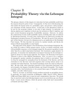
Fig. 1. Flowchart of the SA algorithm
The SA algorithm is represented by the flowchart of Fig. 1. The main feature of SA is its
ability to escape from local optimum based on the acceptance rule of a candidate solution. If
the current solution (f
new
) has an objective function value smaller (supposing minimization)

than that of the old solution (f
old
), then the current solution is accepted. Otherwise, the
current solution can also be accepted if the value given by the Boltzmann distribution:




new old
f f
T
e (1)

is greater than a uniform random number in [0,1], where T is the ‘temperature’ control
parameter. However, many implementation details are left open to the application designer
and are briefly discussed on the following.

2.1 Initial population
Every iterative technique requires definition of an initial guess for parameters’ values. Some
algorithms require the use of several initial solutions but it is not the case of SA. Another
approach is to randomly select the initial parameters’ values given a set of appropriated
boundaries. Of course that as closer the initial estimate is from the global optimum the faster
will be the optimization process.

2.2 Initial temperature
The control parameter ‘temperature’ must be carefully defined since it controls the
acceptance rule defined by (1).
T must be large enough to enable the algorithm to move off a
local minimum but small enough not to move off a global minimum. The value of
T must be

defined in an application based approach since it is related with the magnitude of the
objective function values. It can be found in literature (Pham & Karaboga, 2000) some
empirical approaches that can be helpful not to choose the ‘optimum’ value of
T but at least
a good initial estimate that can be tuned.

2.3 Perturbation mechanism
The perturbation mechanism is the method to create new solutions from the current
solution. In other words it is a method to explore the neighborhood of the current solution
creating small changes in the current solution. SA is commonly used in combinatorial
problems where the parameters being optimized are integer numbers. In an application
where the parameters vary continuously, which is the case of the application presented in
this chapter, the exploration of neighborhood solutions can be made as presented next.
A solution s is defined as a vector s = (
x
1
, , x
n
) representing a point in the search space. A
new solution is generated using a vector σ = (σ
1
, , σ
n
) of standard deviations to create a
perturbation from the current solution. A neighbor solution is then produced from the
present solution by:







 
1
0,
i i i
x x N
(2)

where N(0, σ
i
) is a random Gaussian number with zero mean and σ
i
standard deviation.
Parameter identication of power semiconductor device models using metaheuristics 3
2. Simulated Annealing
Annealing is the metallurgical process of heating up a solid and then cooling slowly until it
crystallizes. Atoms of this material have high energies at very high temperatures. This gives
the atoms a great deal of freedom in their ability to restructure themselves. As the
temperature is reduced the energy of these atoms decreases, until a state of minimum
energy is achieved. In an optimization context SA seeks to emulate this process. SA begins at
a very high temperature where the input values are allowed to assume a great range of
variation. As algorithm progresses temperature is allowed to fall. This restricts the degree to
which inputs are allowed to vary. This often leads the algorithm to a better solution, just as a
metal achieves a better crystal structure through the actual annealing process. So, as long as
temperature is being decreased, changes are produced at the inputs, originating successive
better solutions given rise to an optimum set of input values when temperature is close to
zero. SA can be used to find the minimum of an objective function and it is expected that the
algorithm will find the inputs that will produce a minimum value of the objective function.
In this chapter’s context the goal is to get the optimum set of parameters that produce

realistic and precise simulation results. So, the objective function is an expression that
measures the error between experimental and simulated data.
The main feature of SA algorithm is the ability to avoid being trapped in local minimum.
This is done letting the algorithm to accept not only better solutions but also worse solutions
with a given probability. The main disadvantage, that is common in stochastic local search
algorithms, is that definition of some control parameters (initial temperature, cooling rate,
etc) is somewhat subjective and must be defined from an empirical basis. This means that
the algorithm must be tuned in order to maximize its performance.

Fig. 1. Flowchart of the SA algorithm
The SA algorithm is represented by the flowchart of Fig. 1. The main feature of SA is its
ability to escape from local optimum based on the acceptance rule of a candidate solution. If
the current solution (f
new
) has an objective function value smaller (supposing minimization)
than that of the old solution (f
old
), then the current solution is accepted. Otherwise, the
current solution can also be accepted if the value given by the Boltzmann distribution:




new old
f f
T
e (1)

is greater than a uniform random number in [0,1], where T is the ‘temperature’ control
parameter. However, many implementation details are left open to the application designer

and are briefly discussed on the following.

2.1 Initial population
Every iterative technique requires definition of an initial guess for parameters’ values. Some
algorithms require the use of several initial solutions but it is not the case of SA. Another
approach is to randomly select the initial parameters’ values given a set of appropriated
boundaries. Of course that as closer the initial estimate is from the global optimum the faster
will be the optimization process.

2.2 Initial temperature
The control parameter ‘temperature’ must be carefully defined since it controls the
acceptance rule defined by (1).
T must be large enough to enable the algorithm to move off a
local minimum but small enough not to move off a global minimum. The value of
T must be
defined in an application based approach since it is related with the magnitude of the
objective function values. It can be found in literature (Pham & Karaboga, 2000) some
empirical approaches that can be helpful not to choose the ‘optimum’ value of
T but at least
a good initial estimate that can be tuned.

2.3 Perturbation mechanism
The perturbation mechanism is the method to create new solutions from the current
solution. In other words it is a method to explore the neighborhood of the current solution
creating small changes in the current solution. SA is commonly used in combinatorial
problems where the parameters being optimized are integer numbers. In an application
where the parameters vary continuously, which is the case of the application presented in
this chapter, the exploration of neighborhood solutions can be made as presented next.
A solution s is defined as a vector s = (
x

1
, , x
n
) representing a point in the search space. A
new solution is generated using a vector σ = (σ
1
, , σ
n
) of standard deviations to create a
perturbation from the current solution. A neighbor solution is then produced from the
present solution by:






 
1
0,
i i i
x x N
(2)

where N(0, σ
i
) is a random Gaussian number with zero mean and σ
i
standard deviation.
Simulated Annealing Theory with Applications4

2.4 Objective function
The cost or objective function is an expression that, in some applications, relates the
parameters with some property (distance, cost, etc.) that is desired to minimize or maximize.
In other applications, such as the one presented in this chapter, it is not possible to construct
an objective function that directly relates the model parameters. The approach consists in
defining an objective function that compares simulation results with experimental results.
So, the algorithm will try to find the set of parameters that minimizes the error between
simulated and experimental. Using the normalized sum of the squared errors, the objective
function is expressed by:


 


 
 
 

2
( ) ( )
( )
s i e i
obj
e i
c i
g x g x
f
g x
(3)

where
g
s
(x
i
) is the simulated data, g
e
(x
i
) is the experimental data and c is the number of
curves being optimized.

2.5 Cooling schedule
The most common cooling schedule is the geometric rule for temperature variation:




1i i
T sT
(4)

whit
s < 1. Good results have been report in literature when s is in the range [0.8 , 0.99].
However many other schedules have been proposed in literature. An interesting review is
made in (Fouskakis & Draper, 2002).
Another parameter is the number of iterations at each temperature, which is often related
with the size of the search space or with the size of the neighborhood. This number of
iterations can even be constant or alternatively being function of the temperature or based
on feedback from the process.

2.6 Terminating criterion
There are several methods to control termination of the algorithm. Some criterion examples
are:
a) maximum number of iterations;
b) minimum temperature value;
c) minimum value of objective function;
d) minimum value of acceptance rate.

3. Modeling power semiconductor devices
Modeling charge carrier distribution in low-doped zones of bipolar power semiconductor
devices is known as one of the most important issues for accurate description of the
dynamic behavior of these devices. The charge carrier distribution can be obtained solving
the Ambipolar Diffusion Equation (ADE). Knowledge of hole/electron concentration in that
region is crucial but it is still a challenge for model designers. The last decade has been very
productive since several important SPICE models have been reported in literature with an
interesting trade-off between accuracy and computation time. By solving the ADE, these
models have a strong physics basis which guarantees an interesting accuracy and have also
the advantage that can be implemented in a standard and widely used circuit simulator
(SPICE) that motivates the industrial community to use device simulations for their circuit
designs.
Two main approaches have been developed in order to solve the ADE. The first was
proposed by Leturcq
et al. (Leturcq et al., 1997) using a series expansion of ADE based on
Fourier transform where carrier distribution is implemented using a circuit with resistors
and capacitors (RC network). This technique has been further developed and applied to
several semiconductor devices in (Kang et al., 2002; Kang et al., 2003a; Kang et al., 2003b;
Palmer et al., 2001; Santi et al., 2001; Wang et al., 2004). The second approach proposed by
Araújo
et al. (Araújo et al., 1997) is based on the ADE solution through a variational

formulation and simplex finite elements. One important advantage of this modeling
approach is its easy implementation into general circuit simulators by means of an electrical
analogy with the resulting system of ordinary differential equations (ODEs). ADE
implementation is made with a set of current controlled RC nets which solution is analogue
to the system of ordinary differential equations that results from ADE formulation. This
approach has been applied to several devices in (Chibante et al., 2008; Chibante et al., 2009a;
Chibante et al., 2009b).
In both approaches, a complete device model is obtained adding a few sub-circuits
modeling other regions of the device: emitter, junctions, space-charge and MOS regions.
According to this hybrid approach it is possible to model the charge carrier distribution with
high accuracy maintaining low execution times.

3.1 ADE solution
This section describes the methodology proposed in (Chibante et al., 2008; Chibante et al.,
2009a; Chibante et al., 2009b) to solve ADE. ADE solution is generally obtained considering
that the charge carrier distribution is approximately one-dimensional along the
n
−
region.
Assuming also high-level injection condition (p ≈ n) in device’s low-doped zone the charge
carrier distribution is given by the well-known ADE:


     

 
 


2

2
, , ,
p
x t
p
x t
p
x t
D
t
x
(5)

with boundary conditions:


 
 

 
 
 

 
,
1
2
p
n
n

p
I
p x t
I
x qA D D
(6)

In (5)-(6) D, D
n
and D
p
are diffusion constants, I
n
and I
p
are electron and hole currents and A
the device’s area. It is shown that ADE can be solved by a variational formulation with
posterior solution using the Finite Element Method (FEM) (Zienkiewicz & Morgan, 1983).

Parameter identication of power semiconductor device models using metaheuristics 5
2.4 Objective function
The cost or objective function is an expression that, in some applications, relates the
parameters with some property (distance, cost, etc.) that is desired to minimize or maximize.
In other applications, such as the one presented in this chapter, it is not possible to construct
an objective function that directly relates the model parameters. The approach consists in
defining an objective function that compares simulation results with experimental results.
So, the algorithm will try to find the set of parameters that minimizes the error between
simulated and experimental. Using the normalized sum of the squared errors, the objective
function is expressed by:

 


 
 
 

2
( ) ( )
( )
s i e i
obj
e i
c i
g x g x
f
g x
(3)

where
g
s
(x
i
) is the simulated data, g
e
(x
i
) is the experimental data and c is the number of

curves being optimized.

2.5 Cooling schedule
The most common cooling schedule is the geometric rule for temperature variation:




1i i
T sT
(4)

whit
s < 1. Good results have been report in literature when s is in the range [0.8 , 0.99].
However many other schedules have been proposed in literature. An interesting review is
made in (Fouskakis & Draper, 2002).
Another parameter is the number of iterations at each temperature, which is often related
with the size of the search space or with the size of the neighborhood. This number of
iterations can even be constant or alternatively being function of the temperature or based
on feedback from the process.

2.6 Terminating criterion
There are several methods to control termination of the algorithm. Some criterion examples
are:
a) maximum number of iterations;
b) minimum temperature value;
c) minimum value of objective function;
d) minimum value of acceptance rate.

3. Modeling power semiconductor devices

Modeling charge carrier distribution in low-doped zones of bipolar power semiconductor
devices is known as one of the most important issues for accurate description of the
dynamic behavior of these devices. The charge carrier distribution can be obtained solving
the Ambipolar Diffusion Equation (ADE). Knowledge of hole/electron concentration in that
region is crucial but it is still a challenge for model designers. The last decade has been very
productive since several important SPICE models have been reported in literature with an
interesting trade-off between accuracy and computation time. By solving the ADE, these
models have a strong physics basis which guarantees an interesting accuracy and have also
the advantage that can be implemented in a standard and widely used circuit simulator
(SPICE) that motivates the industrial community to use device simulations for their circuit
designs.
Two main approaches have been developed in order to solve the ADE. The first was
proposed by Leturcq
et al. (Leturcq et al., 1997) using a series expansion of ADE based on
Fourier transform where carrier distribution is implemented using a circuit with resistors
and capacitors (RC network). This technique has been further developed and applied to
several semiconductor devices in (Kang et al., 2002; Kang et al., 2003a; Kang et al., 2003b;
Palmer et al., 2001; Santi et al., 2001; Wang et al., 2004). The second approach proposed by
Araújo
et al. (Araújo et al., 1997) is based on the ADE solution through a variational
formulation and simplex finite elements. One important advantage of this modeling
approach is its easy implementation into general circuit simulators by means of an electrical
analogy with the resulting system of ordinary differential equations (ODEs). ADE
implementation is made with a set of current controlled RC nets which solution is analogue
to the system of ordinary differential equations that results from ADE formulation. This
approach has been applied to several devices in (Chibante et al., 2008; Chibante et al., 2009a;
Chibante et al., 2009b).
In both approaches, a complete device model is obtained adding a few sub-circuits
modeling other regions of the device: emitter, junctions, space-charge and MOS regions.
According to this hybrid approach it is possible to model the charge carrier distribution with

high accuracy maintaining low execution times.

3.1 ADE solution
This section describes the methodology proposed in (Chibante et al., 2008; Chibante et al.,
2009a; Chibante et al., 2009b) to solve ADE. ADE solution is generally obtained considering
that the charge carrier distribution is approximately one-dimensional along the
n
−
region.
Assuming also high-level injection condition (p ≈ n) in device’s low-doped zone the charge
carrier distribution is given by the well-known ADE:


     

 
 


2
2
, , ,
p
x t
p
x t
p
x t
D
t

x
(5)

with boundary conditions:


 
 

 
 
 

 
,
1
2
p
n
n
p
I
p x t
I
x qA D D
(6)

In (5)-(6) D, D
n
and D

p
are diffusion constants, I
n
and I
p
are electron and hole currents and A
the device’s area. It is shown that ADE can be solved by a variational formulation with
posterior solution using the Finite Element Method (FEM) (Zienkiewicz & Morgan, 1983).

Simulated Annealing Theory with Applications6


w
i







T
h
s
ys



w
h

A
ac
c
de
ar
e
pr
e
w
i

Fi
g

i
th:
 
 
G
h
e s
y
mmetr
y
of t
h
s
tem of equation
s
h

ere volta
g
es in
e
normalization c
o
c
eptable values.
R
fined b
y
[I] in fi
r
e
defined specifi
c
e
sented formula
t
i
dth of each finit
e
g
. 2. FEM electric
a


 
 



M

 
 
M














2 2
2 4
2
e
Ee
A
L
 

 

 

F
f
h
ese matrices e
n
s
of a RC networ
k
 




C
e
ach node repres
e
o
nstant (10
17
) is
u
R
esistors values
a
r
st and last node
s

c
all
y
to the t
y
pe
o
t
ion are illustrat
e
e
element.
a
l equivalent cir
c



 
 
 
 



( )
( )
p t
G
p

t
t











2 1
1 4
1
6
1
e Ee
A L
D







 





 
2
2 4 2
2 2
A

1
( ) 0 0
f
t A
n
ables to solve t
h
k
:
  


 



( )
( )
v t
G v t
t

e
nt carrier conce
n
u
sed in order to l
i
a
re defined b
y
[
G
s
implement bou
n
o
f device bein
g

m
e
d in Fig. 2 whe
r
c
uit implementin
g
 
   
   
0F











1
1
4 1
1 2










 
2 1
1 4 1
6
1
e Ee

A
L
D




1
( )
n
g
t A

e s
y
stem (7) ma
k
   

 0I

n
tration alon
g
th
e
i
mit the volta
g
es

G
] and capacitors
n
dar
y
condition
s
m
odeled. Corres
p
r
e A
e
and L
Ee
are
,
g
ADE









4 1

1 2

k
in
g
an analo
gy

e
n
−
zone of the
d

in IsSpice simul
a
b
y
[C]. Current s
s
accordin
g
l
y
to
(
p
ondin
g
RC nets

f
,
respectively, ar
e
(7)
(8)
(9)
(10)
with a
(11)
d
evice.
a
tor to
ources
(
6) and
f
or the
e
a and

R
e



3.
2
T

h
20
0
re
l
m
a
ill
u
Fi
g

3.
2
In

de
m
o
de



3.
2
T
h
th
e
ca

r



e
lated values of r
e
2
IGBT model
h
is section briefl
y
0
9b) with a n
o
l
ationship betwe
e
a
kin
g
clear the
m
u
strates the struc
t
g
. 3. Structure of
a
2

.1 ADE bound
a

order to comp
l
fined, accordin
g
o
deled with the
vice and
T
I
is t
h
2
.2 Emitter mod
e
h
e contribution o
f
e
or
y
of "h" para
m
r
rier stora
g
e re
g

i
o
e
sistors and capa
c




6
6
6
e
ij
ij
A
C
R
D
A
y
presents a com
p
o
n-punch-throu
g
e
n the ADE for
m
m

odel parameter
s
t
ure of an NPT-I
G
a
NPT-IGBT
a
ry conditions
l
ete the ADE f
o
g
l
y
to the devic
e
"h" parameter t
h
h
e total current. S
o
e
l
f
the carrier con
c
m
eters for hi
g

h
o
n:
c
itors are:

 

2
;
6
;
Ee
i j
Ee
i
e e Ee
L
C C
D
D L
R
A
A L
p
lete IGBT mod
e
g
h structure (
N

m
ulation and re
m
s
that will be id
G
BT.
o
rmulation appr
e
bein
g
modele
d
h
eor
y
,
r
n
I
is the

o
, boundar
y
con
d











l
r
p p
x Xl
n T
p
x Xl
n n
x Xr
p
T
n
x Xr
I I
I I I
I I
I I I
c
entration for th
e
doped emitters,


2
0
l
n p
I qh Ap

 
2
2
e Ee
j
e Ee
A L
D
D
R
A L

e
l (Chibante et a
l
N
PT-IGBT) in o
r
m
ainin
g
device
s
e

ntified usin
g
t
h
opriate bounda
r
d
. Current
l
p
I
is

channel current

d
itions (6) are de
f
l
r
p
n

e
total current i
s
assumin
g
a hi
gh

l
., 2008; Chibant
e
r
der to illustra
t
s
ub-models, as
w
h
e SA al
g
orithm.


ry
conditions m
u
a recombinatio
n

from MOS part

f
ined considerin
g
s
well described
h

in
j
ection level
(12)
e
et al.,
t
e the
w
ell as

Fig. 3
u
st be
n
term

of the
g
:
(13)
by the
in the
(14)
Parameter identication of power semiconductor device models using metaheuristics 7


w
i

T
h
s
ys



w
h
A
ac
c
de
ar
e
pr
e
w
i

Fi
g

i

th:




G
h
e s
y
mmetr
y
of t
h
s
tem of equation
s
h
ere volta
g
es in
e
normalization c
o
c
eptable values.
R
fined b
y
[I] in fi
r

e
defined specifi
c
e
sented formula
t
i
dth of each finit
e
g
. 2. FEM electric
a








M





M















2 2
2 4
2
e
Ee
A
L



 
 

F
f
h
ese matrices e
n
s

of a RC networ
k
 




C
e
ach node repres
e
o
nstant (10
17
) is
u
R
esistors values
a
r
st and last node
s
c
all
y
to the t
y
pe
o
t

ion are illustrat
e
e
element.
a
l equivalent cir
c





 
 





( )
( )
p t
G
p
t
t












2 1
1 4
1
6
1
e Ee
A L
D







 




 
2
2 4 2

2 2
A

1
( ) 0 0
f
t A
n
ables to solve t
h
k
:
  


 



( )
( )
v t
G v t
t
e
nt carrier conce
n
u
sed in order to l
i

a
re defined b
y
[
G
s
implement bou
n
o
f device bein
g

m
e
d in Fig. 2 whe
r
c
uit implementin
g
 
   
   
0F












1
1
4 1
1 2










 
2 1
1 4 1
6
1
e Ee
A
L
D





1
( )
n
g
t A

e s
y
stem (7) ma
k
   

 0I

n
tration alon
g
th
e
i
mit the volta
g
es

G
] and capacitors
n
dar
y

condition
s
m
odeled. Corres
p
r
e A
e
and L
Ee
are
,
g
ADE









4 1
1 2

k
in
g
an analo

gy

e
n
−
zone of the
d

in IsSpice simul
a
b
y
[C]. Current s
s
accordin
g
l
y
to
(
p
ondin
g
RC nets
f
,
respectively, ar
e
(7)
(8)

(9)
(10)
with a
(11)
d
evice.
a
tor to
ources
(
6) and
f
or the
e
a and

R
e



3.
2
T
h
20
0
re
l
m

a
ill
u
Fi
g

3.
2
In

de
m
o
de



3.
2
T
h
th
e
ca
r



e
lated values of r

e
2
IGBT model
h
is section briefl
y
0
9b) with a n
o
l
ationship betwe
e
a
kin
g
clear the
m
u
strates the struc
t
g
. 3. Structure of
a
2
.1 ADE bound
a

order to comp
l
fined, accordin

g
o
deled with the
vice and
T
I
is t
h
2
.2 Emitter mod
e
h
e contribution o
f
e
or
y
of "h" para
m
r
rier stora
g
e re
g
i
o
e
sistors and capa
c


 

6
6
6
e
ij
ij
A
C
R
D
A
y
presents a com
p
o
n-punch-throu
g
e
n the ADE for
m
m
odel parameter
s
t
ure of an NPT-I
G
a
NPT-IGBT

a
ry conditions
l
ete the ADE f
o
g
l
y
to the devic
e
"h" parameter t
h
h
e total current. S
o
e
l
f
the carrier con
c
m
eters for hi
g
h
o
n:
c
itors are:

 


2
;
6
;
Ee
i j
Ee
i
e e Ee
L
C C
D
D L
R
A
A L
p
lete IGBT mod
e
g
h structure (
N
m
ulation and re
m
s
that will be id
G
BT.

o
rmulation appr
e
bein
g
modele
d
h
eor
y
,
r
n
I
is the

o
, boundar
y
con
d





 

 
l

r
p p
x Xl
n T
p
x Xl
n n
x Xr
p
T
n
x Xr
I I
I I I
I I
I I I
c
entration for th
e
doped emitters,

2
0
l
n p
I qh Ap

 
2
2

e Ee
j
e Ee
A L
D
D
R
A L

e
l (Chibante et al
N
PT-IGBT) in o
r
m
ainin
g
device
s
e
ntified usin
g
t
h
opriate bounda
r
d
. Current
l
p

I
is

channel current

d
itions (6) are de
f
l
r
p
n

e
total current i
s
assumin
g
a hi
gh

l
., 2008; Chibant
e
r
der to illustra
t
s
ub-models, as
w

h
e SA al
g
orithm.


ry
conditions m
u
a recombinatio
n

from MOS part

f
ined considerin
g
s
well described
h
in
j
ection level
(12)
e
et al.,
t
e the
w
ell as

Fig. 3
u
st be
n
term

of the
g
:
(13)
by the
in the
(14)
Simulated Annealing Theory with Applications8
That relates electron current
l
n
I to carrier concentration at left border of the n
-
region (p
0
).
Emitter zone is seen as a recombination surface that models the recombination process of
electrons that penetrate p
+
region due to limited emitter injection efficiency.

3.2.3 MOSFET model
The MOS part of the device is well represented with standard MOS models, where the

channel current is given by:


 
 

 
 
   
 
 
 
2
2
1
f ds
mos p f gs th ds
gs th
K V
M
I K K V V V
V V
(15)

for triode region and:


 
 



 
 
2
2
1
p gs th
mos
g
s th
K V V
M
I
V V
(16)

for saturation region.
Transient behaviour is ruled by capacitances between device terminals. Well-known
nonlinear Miller capacitance is the most important one in order to describe switching
behaviour of MOS part. It is comprehended of a series combination of gate-drain oxide
capacitance (C
ox
) and gate-drain depletion capacitance (C
gdj
) resulting in the following
expression:






'
1
ox
gd
sc ox
si
g
d
C
C
W C
A
(17)
Drain-source capacitance (C
ds
) is defined as:



si ds
ds
sc
A
C
W
(18)

Gate-source capacitance is normally extracted from capacitance curves and a constant value
may be used.

3.2.4 Voltage drops
As the global model behaves like a current controlled voltage source it is necessary to
evaluate voltage drops over the several regions of the IGBT. Thus, neglecting the
contribution of the high- doped zones (emitter and collector) the total voltage drop (forward
bias) across the device is composed by the following terms:


 

  
IGBT sc
p n
V V V V
(19)
The p
+
n
-
junction voltage drop can be calculated according to Boltzmann approximation:


 
 

 
 
 
2
0

2
ln
T
p n
i
p
V V
n
(20)

Voltage drop across the lightly doped storage region is described integrating electrical field.
Assuming a uniform doping level and quasi-neutrality (n = p + N
D
) over the n
-
zone, and
neglecting diffusion current, we have:


  


 

1
( )
r
l
x
n p n D

x
J
V dx
q p N
(21)

Equation (21) can be seen as a voltage drop across conductivity modulated resistance.
Applying the FEM formulation and using the mean value of p in each finite element results:


  



 



 





1
1
( )
2
r
e

T
e e
e
e n p n D
l
V I
p p
qA N
(22)

Voltage drop over the space charge region is calculated by integrating Poisson equation. For
a uniformly doped base the classical expression is:




 
 
 
 
 
2
2
2
D
si bi
sc sc sc
si D
qN
V

V W W
qN
(23)

3.3 Parameter identification procedure
Identification of semiconductor model parameters will be presented using the NPT-IGBT as
case study. The NPT-IGBT model has been presented in previous section. The model is
characterized by a set of well known physical constants and a set of parameters listed in
Table 1 (Chibante et al., 2009b). This is the set of parameters that must be accurately
identified in order to get precise simulation results. As proposed in this chapter, the
parameters will be identified using the SA optimization algorithm. If the optimum
parameter set produces simulation results that differ from experimental results by an
acceptable error, and in a wide range of operating conditions, then one can conclude that
obtained parameters’ values correspond to the real ones.
It is proposed in (Chibante et al., 2004; Chibante et al., 2009b) to use as experimental data
results from DC analysis and transient analysis. Given the large number of parameters, it
was also suggested to decompose the optimization process in two stages. To accomplish that
the set of parameters is divided in two groups and optimized separately: a first set of
parameters is extracted using the DC characteristic while the second set is extracted using
transient switching waveforms with the optimum parameters from DC extraction. Table 1
presents also the proposed parameter division where the parameters that strongly
Parameter identication of power semiconductor device models using metaheuristics 9
That relates electron current
l
n
I to carrier concentration at left border of the n
-
region (p
0
).

Emitter zone is seen as a recombination surface that models the recombination process of
electrons that penetrate p
+
region due to limited emitter injection efficiency.

3.2.3 MOSFET model
The MOS part of the device is well represented with standard MOS models, where the
channel current is given by:


 
 

 
 
   
 
 
 
2
2
1
f ds
mos p f gs th ds
gs th
K V
M
I K K V V V
V V
(15)

for triode region and:


 
 


 
 
2
2
1
p gs th
mos
g
s th
K V V
M
I
V V
(16)

for saturation region.
Transient behaviour is ruled by capacitances between device terminals. Well-known
nonlinear Miller capacitance is the most important one in order to describe switching
behaviour of MOS part. It is comprehended of a series combination of gate-drain oxide
capacitance (C
ox
) and gate-drain depletion capacitance (C

gdj
) resulting in the following
expression:





'
1
ox
gd
sc ox
si
g
d
C
C
W C
A
(17)
Drain-source capacitance (C
ds
) is defined as:



si ds
ds
sc

A
C
W
(18)

Gate-source capacitance is normally extracted from capacitance curves and a constant value
may be used.

3.2.4 Voltage drops
As the global model behaves like a current controlled voltage source it is necessary to
evaluate voltage drops over the several regions of the IGBT. Thus, neglecting the
contribution of the high- doped zones (emitter and collector) the total voltage drop (forward
bias) across the device is composed by the following terms:


 


 
IGBT sc
p n
V V V V
(19)
The p
+
n
-
junction voltage drop can be calculated according to Boltzmann approximation:

 
 

 
 
 
2
0
2
ln
T
p n
i
p
V V
n
(20)

Voltage drop across the lightly doped storage region is described integrating electrical field.
Assuming a uniform doping level and quasi-neutrality (n = p + N
D
) over the n
-
zone, and
neglecting diffusion current, we have:


  



 

1
( )
r
l
x
n p n D
x
J
V dx
q p N
(21)

Equation (21) can be seen as a voltage drop across conductivity modulated resistance.
Applying the FEM formulation and using the mean value of p in each finite element results:


  



 

 
 
 
 

1

1
( )
2
r
e
T
e e
e
e n p n D
l
V I
p p
qA N
(22)

Voltage drop over the space charge region is calculated by integrating Poisson equation. For
a uniformly doped base the classical expression is:




 
 
 
 
 
2
2
2
D

si bi
sc sc sc
si D
qN
V
V W W
qN
(23)

3.3 Parameter identification procedure
Identification of semiconductor model parameters will be presented using the NPT-IGBT as
case study. The NPT-IGBT model has been presented in previous section. The model is
characterized by a set of well known physical constants and a set of parameters listed in
Table 1 (Chibante et al., 2009b). This is the set of parameters that must be accurately
identified in order to get precise simulation results. As proposed in this chapter, the
parameters will be identified using the SA optimization algorithm. If the optimum
parameter set produces simulation results that differ from experimental results by an
acceptable error, and in a wide range of operating conditions, then one can conclude that
obtained parameters’ values correspond to the real ones.
It is proposed in (Chibante et al., 2004; Chibante et al., 2009b) to use as experimental data
results from DC analysis and transient analysis. Given the large number of parameters, it
was also suggested to decompose the optimization process in two stages. To accomplish that
the set of parameters is divided in two groups and optimized separately: a first set of
parameters is extracted using the DC characteristic while the second set is extracted using
transient switching waveforms with the optimum parameters from DC extraction. Table 1
presents also the proposed parameter division where the parameters that strongly
Simulated Annealing Theory with Applications10
influences DC characteristics were selected in order to run the DC optimization. In the
following sections the first optimization stage will be referred as DC optimization and the
second as transient optimization.

Table 1. List of NPT-IGBT model parameters

4. Simulated Annealing implementation
As described in section two of this chapter, application of the SA algorithm requires
definition of:

a)
Initial population;
b)
Initial temperature;
c)
Perturbation mechanism;
d)
Objective function;
e)
Cooling schedule;
f)
Terminating criterion.

SA algorithm has a disadvantage that is common to most metaheuristics in the sense that
many implementation aspects are left open to the designer and many algorithm controls are
defined in an ad-hoc basis or are the result of a tuning stage. In the following it is presented
the approach suggested in (Chibante et al., 2009b).

4.1 Initial population
Every iterative technique requires definition of an initial guess for parameters’ values. Some
algorithms require the use of several initial parameter sets but it is not the case of SA.
Another approach is to randomly select the initial parameters’ values given a set of
appropriated boundaries. Of course that as closer the initial estimate is from the global

optimum the faster will be the optimization process. The approach proposed in (Chibante et
Optimization

Symbol Unit Description
Transient
A
gd

cm² Gate-drain overlap area
W
B

cm Metallurgical base width
N
B

cm
-
³ Base doping concentration
V
bi

V Junction in-built voltage
C
gs

F Gate-source capacitance
C
oxd

F Gate-drain overlap oxide capacitance
DC
A
cm² Device active area
h
p

cm
4
.s
-1
Recombination parameter
K
f

- Triode region MOSFET transconductance factor
K
p

A/V² Saturation region MOSFET transconductance
V
th

V MOSFET channel threshold voltage
τ
s Base lifetime


V
-

¹ Transverse field transconductance factor
al., 2009b) is to use some well know techniques (Chibante et al., 2004; Kang et al., 2003c;
Leturcq et al., 1997) to find an interesting initial solution for some of the parameters. These
simple techniques are mainly based in datasheet information or known relations between
parameters. Since this family of optimization techniques requires a tuning process, in the
sense that algorithm control variables must be refined to maximize algorithm performance,
the initial solution can also be tuned if some of parameter if clearly far way from expected
global optimum.

4.2 Initial temperature
As stated before, the temperature must be large enough to enable the algorithm to move off
a local minimum but small enough not to move off a global minimum. This is related to the
acceptance probability of a worst solution that depends on temperature and magnitude of
objective function. In this context, the algorithm was tuned and the initial temperature was
set to 1.

4.3 Perturbation mechanism
A solution x is defined as a vector x = (x
1
, , x
n
) representing a point in the search space. A
new solution is generated using a vector
σ = (σ
1
, , σ
n
) of standard deviations to create a
perturbation from the current solution. A neighbor solution is then produced from the
present solution by:





 
1
0,
i i i
x x N
(24)

where N(0, σ
i
) is a random Gaussian number with zero mean and σ
i
standard deviation. The
construction of the vector
σ requires definition of a value σ
i
related to each parameter x
i
.
That depends on the confidence used to construct the initial solution, in sense that if there is
a high confidence that a certain parameter is close to a certain value, then the corresponding
standard deviation can be set smaller. In a more advanced scheme the vector
σ can be made
variable by a constant rate as a function of the number of iterations or based in acceptance
rates (Pham & Karaboga, 2000). No constrains were imposed to the parameter variation,

which means that there is no lower or upper bounds.

4.4 Objective function
The cost or objective function is defined by comparing the relative error between simulated
and experimental data using the normalized sum of the squared errors. The general
expression is:


 


 
 
 

2
( ) ( )
( )
s i e i
obj
e i
c i
g x g x
f
g x
(25)

where g
s
(x

i
) is the simulated data, g
e
(x
i
) is the experimental data and c is the number of
curves being optimized. The IGBT’s DC characteristic is used as optimization variable for
the DC optimization. This characteristic relates collector current to collector-emitter voltage
Parameter identication of power semiconductor device models using metaheuristics 11
influences DC characteristics were selected in order to run the DC optimization. In the
following sections the first optimization stage will be referred as DC optimization and the
second as transient optimization.

Table 1. List of NPT-IGBT model parameters

4. Simulated Annealing implementation
As described in section two of this chapter, application of the SA algorithm requires
definition of:

a)
Initial population;
b)
Initial temperature;
c)
Perturbation mechanism;
d)
Objective function;
e)
Cooling schedule;
f)

Terminating criterion.

SA algorithm has a disadvantage that is common to most metaheuristics in the sense that
many implementation aspects are left open to the designer and many algorithm controls are
defined in an ad-hoc basis or are the result of a tuning stage. In the following it is presented
the approach suggested in (Chibante et al., 2009b).

4.1 Initial population
Every iterative technique requires definition of an initial guess for parameters’ values. Some
algorithms require the use of several initial parameter sets but it is not the case of SA.
Another approach is to randomly select the initial parameters’ values given a set of
appropriated boundaries. Of course that as closer the initial estimate is from the global
optimum the faster will be the optimization process. The approach proposed in (Chibante et
Optimization

Symbol Unit Description
Transient
A
gd

cm² Gate-drain overlap area
W
B

cm Metallurgical base width
N
B

cm
-

³ Base doping concentration
V
bi

V Junction in-built voltage
C
gs

F Gate-source capacitance
C
oxd

F Gate-drain overlap oxide capacitance
DC
A
cm² Device active area
h
p

cm
4
.s
-1
Recombination parameter
K
f

- Triode region MOSFET transconductance factor
K
p

A/V² Saturation region MOSFET transconductance
V
th

V MOSFET channel threshold voltage
τ
s Base lifetime


V
-
¹ Transverse field transconductance factor
al., 2009b) is to use some well know techniques (Chibante et al., 2004; Kang et al., 2003c;
Leturcq et al., 1997) to find an interesting initial solution for some of the parameters. These
simple techniques are mainly based in datasheet information or known relations between
parameters. Since this family of optimization techniques requires a tuning process, in the
sense that algorithm control variables must be refined to maximize algorithm performance,
the initial solution can also be tuned if some of parameter if clearly far way from expected
global optimum.

4.2 Initial temperature
As stated before, the temperature must be large enough to enable the algorithm to move off
a local minimum but small enough not to move off a global minimum. This is related to the
acceptance probability of a worst solution that depends on temperature and magnitude of
objective function. In this context, the algorithm was tuned and the initial temperature was
set to 1.

4.3 Perturbation mechanism
A solution x is defined as a vector x = (x

1
, , x
n
) representing a point in the search space. A
new solution is generated using a vector
σ = (σ
1
, , σ
n
) of standard deviations to create a
perturbation from the current solution. A neighbor solution is then produced from the
present solution by:






 
1
0,
i i i
x x N
(24)

where N(0, σ
i
) is a random Gaussian number with zero mean and σ
i
standard deviation. The

construction of the vector
σ requires definition of a value σ
i
related to each parameter x
i
.
That depends on the confidence used to construct the initial solution, in sense that if there is
a high confidence that a certain parameter is close to a certain value, then the corresponding
standard deviation can be set smaller. In a more advanced scheme the vector
σ can be made
variable by a constant rate as a function of the number of iterations or based in acceptance
rates (Pham & Karaboga, 2000). No constrains were imposed to the parameter variation,
which means that there is no lower or upper bounds.

4.4 Objective function
The cost or objective function is defined by comparing the relative error between simulated
and experimental data using the normalized sum of the squared errors. The general
expression is:


 


 
 
 

2
( ) ( )
( )

s i e i
obj
e i
c i
g x g x
f
g x
(25)

where g
s
(x
i
) is the simulated data, g
e
(x
i
) is the experimental data and c is the number of
curves being optimized. The IGBT’s DC characteristic is used as optimization variable for
the DC optimization. This characteristic relates collector current to collector-emitter voltage
Simulated Annealing Theory with Applications12
for several gate-emitter voltages. Three experimental points for three gate-emitter values
were measured to construct the objective function:


 
 


 

 
 

2
3 3
1 1
( ) ( )
( )
s i e i
obj
e i
c i
g x g x
f
g x
(26)

So, a total of 9 data points were used from the experimental DC characteristic g
e
(x
i
) and
compared with the simulated DC characteristic g
e
(x
i
) using (26).
The transient optimization is a more difficult task since it is required that a good simulated
behaviour should be observed either for turn-on and turn-off, considering the three main
variables: collector-emitter voltage (V

CE
), gate-emitter voltage (V
GE
) and collector current
(I
C
). Although optimization using the three main variables (V
CE
, V
GE
, I
C
) could probably lead
to a robust optimization process, it has been observed that optimizing just for V
CE
produces
also good results for remaining variables, as long as the typical current tail phenomenon is
not significant. Collector current by itself is not an adequate optimization variable since the
effects of some phenomenon (namely capacitances) is not readily visible in shape waveform.
Optimization using switching parameters values instead of transient switching waveforms
is also a possible approach (Allard et al., 2003). In the present work collector-emitter voltage
was used as optimization variable in the objective function:



 


 
 

 

2
_ _
_
1
( ) ( )
( )
n
CE s i CE e i
obj
CE e i
i
V t V t
f
V t
(27)

using n data points of experimental (V
CE_e
) and simulated (V
CE_s
) waveforms. It is interesting
to note from the realized experiments that although collector-emitter voltage is optimized
only at turn-off a good agreement is obtained for the whole switching cycle.

4.5 Cooling schedule
The cooling schedule was implemented using a geometric rule for temperature variation:



1i i
T sT
(28)

A value of s = 0.4 was found to give good results.

4.6 Terminating criterion
For a given iteration of the SA algorithm, IsSpice circuit simulator is called in order to run a
simulation with the current trial set of parameters. Implementation of the interaction
between optimization algorithm and IsSpice requires some effort because each parameter
set must be inserted into the IsSpice’s netlist file and output data must be read. The
simulation time is about 1 second for a DC simulation and 15 seconds for a transient
simulation. Objective function is then evaluated with simulated and experimental data
accordingly to (26) and (27). This means that each evaluation of the objective function takes
about 15 seconds in the worst case. This is a disadvantage of the present application since
evaluation of a common objective function usually requires computation of an equation that
is made almost instantaneously. This imposes some limits in the number of algorithm
iterations to avoid extremely long optimization times. So, it was decided to use a maximum
of 100 iterations as terminating criterion for transient optimization and a minimum value of
0.5 for the objective function in the DC optimization.

4.7 Optimization results
Fig. 4 presents the results for the DC optimization. It is clear that simulated DC
characteristic agrees well with the experimental DC characteristic defined by the 9
experimental data points. The experimental data is taken from a BUP203 device
(1000V/23A). Table 2 presents the initial solution and corresponding
σ vector for DC
optimization and the optimum parameter set. Results for the transient optimization are

presented (Fig. 5) concerning the optimization process but also further model validation
results in order to assess the robustness of the extraction optimization process. Experimental
results are from a BUP203 device (1000V/23A) using a test circuit in a hard-switching
configuration with resistive load. Operating conditions are: V
CC
= 150V, R
L
= 20Ω and gate
resistances R
G1
= 1.34kΩ, R
G2
= 2.65kΩ and R
G3
= 7.92kΩ. Note that the objective function is
evaluated using only the collector-emitter variable with R
G1
= 1.34kΩ. Although collector-
emitter voltage is optimized only at turn-off it is interesting to note that a good agreement is
obtained for the whole switching cycle. Table 3 presents the initial solution and
corresponding
σ vector for transient optimization and the optimum parameter set.


Fig. 4. Experimental and simulated DC characteristics


Parameter
A
(cm²)

h
p

(cm
4
.s
-1
)
K
f

K
p

(A/V²)
V
th

(V)
τ
(µs)

(V
-
¹)
Initial value 0.200 500×10
-14
3.10 0.90×10
-5
4.73 50 12.0×10

-5

Optimum value 0.239 319×10
-14
2.17 0.72×10
-5
4.76 54 8.8×10
-5

Table 2. Initial conditions and final result (DC optimization)
Parameter identication of power semiconductor device models using metaheuristics 13
for several gate-emitter voltages. Three experimental points for three gate-emitter values
were measured to construct the objective function:


 
 


 
 
 

2
3 3
1 1
( ) ( )
( )
s i e i
obj

e i
c i
g x g x
f
g x
(26)

So, a total of 9 data points were used from the experimental DC characteristic g
e
(x
i
) and
compared with the simulated DC characteristic g
e
(x
i
) using (26).
The transient optimization is a more difficult task since it is required that a good simulated
behaviour should be observed either for turn-on and turn-off, considering the three main
variables: collector-emitter voltage (V
CE
), gate-emitter voltage (V
GE
) and collector current
(I
C
). Although optimization using the three main variables (V
CE
, V
GE

, I
C
) could probably lead
to a robust optimization process, it has been observed that optimizing just for V
CE
produces
also good results for remaining variables, as long as the typical current tail phenomenon is
not significant. Collector current by itself is not an adequate optimization variable since the
effects of some phenomenon (namely capacitances) is not readily visible in shape waveform.
Optimization using switching parameters values instead of transient switching waveforms
is also a possible approach (Allard et al., 2003). In the present work collector-emitter voltage
was used as optimization variable in the objective function:



 


 
 
 

2
_ _
_
1
( ) ( )
( )
n
CE s i CE e i

obj
CE e i
i
V t V t
f
V t
(27)

using n data points of experimental (V
CE_e
) and simulated (V
CE_s
) waveforms. It is interesting
to note from the realized experiments that although collector-emitter voltage is optimized
only at turn-off a good agreement is obtained for the whole switching cycle.

4.5 Cooling schedule
The cooling schedule was implemented using a geometric rule for temperature variation:




1i i
T sT
(28)

A value of s = 0.4 was found to give good results.

4.6 Terminating criterion
For a given iteration of the SA algorithm, IsSpice circuit simulator is called in order to run a

simulation with the current trial set of parameters. Implementation of the interaction
between optimization algorithm and IsSpice requires some effort because each parameter
set must be inserted into the IsSpice’s netlist file and output data must be read. The
simulation time is about 1 second for a DC simulation and 15 seconds for a transient
simulation. Objective function is then evaluated with simulated and experimental data
accordingly to (26) and (27). This means that each evaluation of the objective function takes
about 15 seconds in the worst case. This is a disadvantage of the present application since
evaluation of a common objective function usually requires computation of an equation that
is made almost instantaneously. This imposes some limits in the number of algorithm
iterations to avoid extremely long optimization times. So, it was decided to use a maximum
of 100 iterations as terminating criterion for transient optimization and a minimum value of
0.5 for the objective function in the DC optimization.

4.7 Optimization results
Fig. 4 presents the results for the DC optimization. It is clear that simulated DC
characteristic agrees well with the experimental DC characteristic defined by the 9
experimental data points. The experimental data is taken from a BUP203 device
(1000V/23A). Table 2 presents the initial solution and corresponding
σ vector for DC
optimization and the optimum parameter set. Results for the transient optimization are
presented (Fig. 5) concerning the optimization process but also further model validation
results in order to assess the robustness of the extraction optimization process. Experimental
results are from a BUP203 device (1000V/23A) using a test circuit in a hard-switching
configuration with resistive load. Operating conditions are: V
CC
= 150V, R
L
= 20Ω and gate
resistances R
G1

= 1.34kΩ, R
G2
= 2.65kΩ and R
G3
= 7.92kΩ. Note that the objective function is
evaluated using only the collector-emitter variable with R
G1
= 1.34kΩ. Although collector-
emitter voltage is optimized only at turn-off it is interesting to note that a good agreement is
obtained for the whole switching cycle. Table 3 presents the initial solution and
corresponding
σ vector for transient optimization and the optimum parameter set.


Fig. 4. Experimental and simulated DC characteristics


Parameter
A
(cm²)
h
p

(cm
4
.s
-1
)
K
f

K
p

(A/V²)
V
th

(V)
τ
(µs)

(V
-
¹)
Initial value 0.200 500×10
-14
3.10 0.90×10
-5
4.73 50 12.0×10
-5

Optimum value 0.239 319×10
-14
2.17 0.72×10
-5
4.76 54 8.8×10
-5

Table 2. Initial conditions and final result (DC optimization)

Simulated Annealing Theory with Applications14

Fig. 5. Experimental and simulated (bold) transient curves at turn-on (left) and turn-off

Parameter
A
gd

(cm²)
C
gs

(nF)
C
oxd

(nF)
N
B

(cm
-
³)
V
bi

(V)
W
B

(cm)
Initial value 0.090 1.80 3.10 0.40×10
14
0.70 18.0×10
-3

Optimum value 0.137 2.46 2.58 0.41×10
14
0.54 20.2×10
-3

Table 3. Initial conditions and final result (transient optimization)

5. Conclusion
An optimization-based methodology is presented to support the parameter identification of
a NPT-IGBT physical model. The SA algorithm is described and applied successfully. The
main features of SA are presented as well as the algorithm design. Using a simple turn-off
test the model performance is maximized corresponding to a set of parameters that
accurately characterizes the device behavior in DC and transient conditions. Accurate power
semiconductor modeling and parameter extraction with reduced CPU time is possible with
proposed approach.

6. References
Allard, B. et al. (2003). Systematic procedure to map the validity range of insulated-gate
device models, Proceedings of 10th European Conference on Power Electronics and
Applications (EPE'03), Toulouse, France, 2003
Araújo, A. et al. (1997). A new approach for analogue simulation of bipolar semiconductors,
Proceedings of the 2nd Brazilian Conference Power Electronics (COBEP'97), pp. 761-765,
Belo-Horizonte, Brasil, 1997
Bryant, A.T. et al. (2006). Two-Step Parameter Extraction Procedure With Formal

Optimization for Physics-Based Circuit Simulator IGBT and p-i-n Diode Models,
IEEE Transactions on Power Electronics, Vol. 21, No. 2, pp. 295-309
Chibante, R. et al. (2004). A simple and efficient parameter extraction procedure for physics
based IGBT models, Proceedings of 11th International Power Electronics and Motion
Control Conference (EPE-PEMC'04), Riga, Latvia, 2004
Chibante, R. et al. (2008). A new approach for physical-based modelling of bipolar power
semiconductor devices, Solid-State Electronics, Vol. 52, No. 11, pp. 1766-1772
Chibante, R. et al. (2009a). Finite element power diode model optimized through experiment
based parameter extraction, International Journal of Numerical Modeling: Electronic
Networks, Devices and Fields, Vol. 22, No. 5, pp. 351-367
Chibante, R. et al. (2009b). Finite-Element Modeling and Optimization-Based Parameter
Extraction Algorithm for NPT-IGBTs, IEEE Transactions on Power Electronics, Vol.
24, No. 5, pp. 1417-1427
Claudio, A. et al. (2002). Parameter extraction for physics-based IGBT models by electrical
measurements, Proceedings of 33rd Annual IEEE Power Electronics Specialists
Conference (PESC'02), Vol. 3, pp. 1295-1300, Cairns, Australia, 2002
Fouskakis, D. & Draper, D. (2002). Stochastic optimization: a review, International Statistical
Review, Vol. 70, No. 3, pp. 315-349
Hefner, A.R. & Bouche, S. (2000). Automated parameter extraction software for advanced
IGBT modeling, 7th Workshop on Computers in Power Electronics (COMPEL'00) pp.
10-18, 2000
Kang, X. et al. (2002). Low temperature characterization and modeling of IGBTs, Proceedings
of 33rd Annual IEEE Power Electronics Specialists Conference (PESC'02), Vol. 3, pp.
1277-1282, Cairns, Australia, 2002
Kang, X. et al. (2003a). Characterization and modeling of high-voltage field-stop IGBTs,
IEEE Transactions on Industry Applications, Vol. 39, No. 4, pp. 922-928
Parameter identication of power semiconductor device models using metaheuristics 15

Fig. 5. Experimental and simulated (bold) transient curves at turn-on (left) and turn-off

Parameter
A
gd

(cm²)
C
gs

(nF)
C
oxd

(nF)
N
B

(cm
-
³)
V
bi

(V)
W
B

(cm)
Initial value 0.090 1.80 3.10 0.40×10
14
0.70 18.0×10

-3

Optimum value 0.137 2.46 2.58 0.41×10
14
0.54 20.2×10
-3

Table 3. Initial conditions and final result (transient optimization)

5. Conclusion
An optimization-based methodology is presented to support the parameter identification of
a NPT-IGBT physical model. The SA algorithm is described and applied successfully. The
main features of SA are presented as well as the algorithm design. Using a simple turn-off
test the model performance is maximized corresponding to a set of parameters that
accurately characterizes the device behavior in DC and transient conditions. Accurate power
semiconductor modeling and parameter extraction with reduced CPU time is possible with
proposed approach.

6. References
Allard, B. et al. (2003). Systematic procedure to map the validity range of insulated-gate
device models, Proceedings of 10th European Conference on Power Electronics and
Applications (EPE'03), Toulouse, France, 2003
Araújo, A. et al. (1997). A new approach for analogue simulation of bipolar semiconductors,
Proceedings of the 2nd Brazilian Conference Power Electronics (COBEP'97), pp. 761-765,
Belo-Horizonte, Brasil, 1997
Bryant, A.T. et al. (2006). Two-Step Parameter Extraction Procedure With Formal
Optimization for Physics-Based Circuit Simulator IGBT and p-i-n Diode Models,
IEEE Transactions on Power Electronics, Vol. 21, No. 2, pp. 295-309
Chibante, R. et al. (2004). A simple and efficient parameter extraction procedure for physics
based IGBT models, Proceedings of 11th International Power Electronics and Motion

Control Conference (EPE-PEMC'04), Riga, Latvia, 2004
Chibante, R. et al. (2008). A new approach for physical-based modelling of bipolar power
semiconductor devices, Solid-State Electronics, Vol. 52, No. 11, pp. 1766-1772
Chibante, R. et al. (2009a). Finite element power diode model optimized through experiment
based parameter extraction, International Journal of Numerical Modeling: Electronic
Networks, Devices and Fields, Vol. 22, No. 5, pp. 351-367
Chibante, R. et al. (2009b). Finite-Element Modeling and Optimization-Based Parameter
Extraction Algorithm for NPT-IGBTs, IEEE Transactions on Power Electronics, Vol.
24, No. 5, pp. 1417-1427
Claudio, A. et al. (2002). Parameter extraction for physics-based IGBT models by electrical
measurements, Proceedings of 33rd Annual IEEE Power Electronics Specialists
Conference (PESC'02), Vol. 3, pp. 1295-1300, Cairns, Australia, 2002
Fouskakis, D. & Draper, D. (2002). Stochastic optimization: a review, International Statistical
Review, Vol. 70, No. 3, pp. 315-349
Hefner, A.R. & Bouche, S. (2000). Automated parameter extraction software for advanced
IGBT modeling, 7th Workshop on Computers in Power Electronics (COMPEL'00) pp.
10-18, 2000
Kang, X. et al. (2002). Low temperature characterization and modeling of IGBTs, Proceedings
of 33rd Annual IEEE Power Electronics Specialists Conference (PESC'02), Vol. 3, pp.
1277-1282, Cairns, Australia, 2002
Kang, X. et al. (2003a). Characterization and modeling of high-voltage field-stop IGBTs,
IEEE Transactions on Industry Applications, Vol. 39, No. 4, pp. 922-928
Simulated Annealing Theory with Applications16
Kang, X. et al. (2003b). Characterization and modeling of the LPT CSTBT - the 5th generation
IGBT, Conference Record of the 38th IAS Annual Meeting, Vol. 2, pp. 982-987, UT,
United States, 2003b
Kang, X. et al. (2003c). Parameter extraction for a physics-based circuit simulator IGBT
model, Proceedings of the 18th Annual IEEE Applied Power Electronics Conference and
Exposition (APEC'03), Vol. 2, pp. 946-952, Miami Beach, FL, United States, 2003c
Lauritzen, P.O. et al. (2001). A basic IGBT model with easy parameter extraction, Proceedings

of 32nd Annual IEEE Power Electronics Specialists Conference (PESC'01), Vol. 4, pp.
2160-2165, Vancouver, BC, Canada, 2001
Leturcq, P. et al. (1997). A distributed model of IGBTs for circuit simulation, Proceedings of
7th European Conference on Power Electronics and Applications (EPE'97), pp. 494-501,
1997
Palmer, P.R. et al. (2001). Circuit simulator models for the diode and IGBT with full
temperature dependent features, Proceedings of 32nd Annual IEEE Power Electronics
Specialists Conference (PESC'01), Vol. 4, pp. 2171-2177, 2001
Pham, D.T. & Karaboga, D. (2000). Intelligent optimisation techniques: genetic algorithms,
tabu search, simulated annealing and neural networks, Springer, New York
Santi, E. et al. (2001). Temperature effects on trench-gate IGBTs, Conference Record of the 36th
IEEE Industry Applications Conference (IAS'01), Vol. 3, pp. 1931-1937, 2001
Wang, X. et al. (2004). Implementation and validation of a physics-based circuit model for
IGCT with full temperature dependencies, Proceedings of 35th Annual IEEE Power
Electronics Specialists Conference (PESC'04), Vol. 1, pp. 597-603, 2004
Zienkiewicz, O.C. & Morgan, K. (1983). Finite elements and aproximations, John Wiley &
Sons, New York



Application of simulated annealing and hybrid methods in
the solution of inverse heat and mass transfer problems 17
Application of simulated annealing and hybrid methods in the solution of
inverse heat and mass transfer problems
Antônio José da Silva Neto, Jader Lugon Junior, Francisco José da Cunha Pires Soeiro,
Luiz Biondi Neto, Cesar Costapinto Santana, Fran Sérgio Lobato and Valder Steffen Junior

x

Application of simulated annealing and

hybrid methods in the solution of inverse
heat and mass transfer problems

Antônio José da Silva Neto
1
,
Jader Lugon Junior
2,5
, Francisco José da Cunha Pires Soeiro
1
,
Luiz Biondi Neto
1
, Cesar Costapinto Santana
3
,
Fran Sérgio Lobato
4
and Valder Steffen Junior
4

Universidade do Estado do Rio de Janeiro
1
,
Instituto Federal de Educação, Ciência e Tecnologia Fluminense
2
,
Universidade Estadual de Campinas
3
,

Universidade Federal de Uberlândia
4
,
Centro de Tecnologia SENAI-RJ Ambiental
5

Brazil

1. Introduction
The problem of parameter identification characterizes a typical inverse problem in
engineering. It arises from the difficulty in building theoretical models that are able to
represent satisfactorily physical phenomena under real operating conditions. Considering
the possibility of using more complex models along with the information provided by
experimental data, the parameters obtained through an inverse problem approach may then
be used to simulate the behavior of the system for different operation conditions.
Traditionally, this kind of problem has been treated by using either classical or deterministic
optimization techniques (Baltes et al., 1994; Cazzador and Lubenova, 1995; Su and Silva
Neto, 2001; Silva Neto and Özişik 1993ab, 1994; Yan et al., 2008; Yang et al., 2009). In the
recent years however, the use of non-deterministic techniques or the coupling of these
techniques with classical approaches thus forming a hybrid methodology became very
popular due to the simplicity and robustness of evolutionary techniques (Wang et al., 2001;
Silva Neto and Soeiro, 2002, 2003; Silva Neto and Silva Neto, 2003; Lobato and Steffen Jr.,
2007; Lobato et al., 2008, 2009, 2010).
The solution of inverse problems has several relevant applications in engineering and
medicine. A lot of attention has been devoted to the estimation of boundary and initial
conditions in heat conduction problems (Alifanov, 1974, Beck et al., 1985, Denisov and
Solov’yera, 1993, Muniz et al., 1999) as well as thermal properties (Artyukhin, 1982,
Carvalho and Silva Neto, 1999, Soeiro et al., 2000; Su and Silva Neto, 2001; Lobato et al.,
2009) and heat source intensities (Borukhov and Kolesnikov, 1988, Silva Neto and Özisik,
1993ab, 1994, Orlande and Özisik, 1993, Moura Neto and Silva Neto, 2000, Wang et al., 2000)

2