SOIL CONTAMINATION pps
Bạn đang xem bản rút gọn của tài liệu. Xem và tải ngay bản đầy đủ của tài liệu tại đây (8.03 MB, 180 trang )
SOIL CONTAMINATION
Edited by Simone Pascucci
Soil Contamination
Edited by Simone Pascucci
Published by InTech
Janeza Trdine 9, 51000 Rijeka, Croatia
Copyright © 2011 InTech
All chapters are Open Access articles distributed under the Creative Commons
Non Commercial Share Alike Attribution 3.0 license, which permits to copy,
distribute, transmit, and adapt the work in any medium, so long as the original
work is properly cited. After this work has been published by InTech, authors
have the right to republish it, in whole or part, in any publication of which they
are the author, and to make other personal use of the work. Any republication,
referencing or personal use of the work must explicitly identify the original source.
Statements and opinions expressed in the chapters are these of the individual contributors
and not necessarily those of the editors or publisher. No responsibility is accepted
for the accuracy of information contained in the published articles. The publisher
assumes no responsibility for any damage or injury to persons or property arising out
of the use of any materials, instructions, methods or ideas contained in the book.
Publishing Process Manager Alenka Urbancic
Technical Editor Teodora Smiljanic
Cover Designer Jan Hyrat
Image Copyright Jostein Hauge, 2010. Used under license from Shutterstock.com
First published August, 2011
Printed in Croatia
A free online edition of this book is available at www.intechopen.com
Additional hard copies can be obtained from
Soil Contamination, Edited by Simone Pascucci
p. cm.
ISBN 978-953-307-647-8
free online editions of InTech
Books and Journals can be found at
www.intechopen.com
Contents
Preface IX
Chapter 1 Long-Term Monitoring of Dioxin
and Furan Level in Soil Around Medical Waste Incinerator 1
Li Xiao-dong, Yan Mi, Chen Tong,
Lu Sheng-yong and Yan Jian-hua
Chapter 2 Research for Investigating
and Managing Soil Contamination
Caused by Winter Maintenance in Cold Regions 19
Helen K. French and Sjoerd E.A.T.M. van der Zee
Chapter 3 Soil-Transmitted Helminthic Zoonoses
in Humans and Associated Risk Factors 43
Vamilton Alvares Santarém, Guita Rubinsky-Elefant
and Marcelo Urbano Ferreira
Chapter 4 Reflectance Spectroscopy
as a Tool for Monitoring Contaminated Soils 67
Guy Schwartz, Gil Eshel and Eyal Ben-Dor
Chapter 5 Multi-Technique Application for
Waste Material Detection and Soil Remediation
Strategies: The Red Mud Dust and Fly Ash Case Studies 91
Claudia Belviso, Simone Pascucci, Francesco Cavalcante,
Angelo Palombo, Stefano Pignatti,
Tiziana Simoniello and Saverio Fiore
Chapter 6 Heavy Metals Contaminated Soils
and Phytoremediation Strategies in Taiwan 107
Hung-Yu Lai, Shaw-Wei Su,
Horng-Yuh Guo and Zueng-Sang Chen
Chapter 7 Biological Remediation of
Hydrocarbon and Heavy Metals Contaminated Soil 127
O. Peter Abioye
VI Contents
Chapter 8 Bioindicators and Biomarkers
in the Assessment of Soil Toxicity 143
Carmem Silvia Fontanetti, Larissa Rosa Nogarol,
Raphael Bastão de Souza, Danielli Giuliano Perez
and Guilherme Thiago Maziviero
Preface
Soil contamination has severely increased over the last years, especially due to
petroleum hydrocarbons, heavy metals and pesticides from industrial wastes and
human activities. Even though in general soil quality research is facing an important
technological challenge and several actions have been taken in order to assess,
remediate and reduce the effects of contaminants on soils, suitable and standardized
monitoring and remediation strategies of soil are required. In this sense, in the last
decade there has been a growing emphasis on the utilization of residues and waste
materials, coming from different industrial activities, in several remediation
technologies (e.g., chemical degradation, photo-degradation) and bioremediation in
order to clean up contaminated soils. The critical point regarding contaminated soil
monitoring is the intrinsic difficulty in defining fixed monitoring variables and
indicators as the establishment of any a priori criterion and threshold for soil quality
can be still considered subjective.
The book aims at collecting contributions from outstanding scientists and experts
involved in different fields of soil contamination in order to show new research
highlights and future developments in the context of contaminated soil monitoring
and remediation strategies. The book is organized into eight auto-consistent chapters
regarding application-oriented studies in the field of soil contamination.
The chapters include selected topics covering long-term monitoring studies of dioxin
and furan level in soils; contamination of factory and roadside soils by hydrocarbons
and heavy metals; soil contamination caused by winter maintenance in cold regions;
the use of reflectance spectroscopy and hyperspectral remote sensing for soil
contaminants and waste material detection; an updated review of the use of
bioindicators and biomarkers for the assessment of soil toxicity and of soil transmitted
pathogens in humans and associated risk factors; and also a consistent review of
different remediation technologies and strategies (bio-phytoremediation) of
contaminated soils.
I hope that the collected materials will provide to soil contamination researchers,
experts (e.g., geologists, engineers and biologists), practitioners at universities, and
other interested end-users a scientific basis and practical guide in the field of soil
contamination to widen their experience to the presented topic areas.
X Preface
All issues regarding soil contamination included in the book are significant and I want
to thanks the authors for their precious contribution.
Dr. Simone Pascucci
CNR - Institute of methodologies for
environmental analysis,
Italy
1
Long-Term Monitoring of Dioxin and Furan
Level in Soil Around Medical Waste Incinerator
Li Xiao-dong, Yan Mi, Chen Tong, Lu Sheng-yong and Yan Jian-hua
State Key Laboratory of Clean Energy Utilization, Zhejiang University
Hangzhou City,
PR China
1. Introduction
The annual generation of solid waste is quite huge in China. For instance, approx. 157
million tons of municipal solid waste (MSW) and 2.04 billion tons of industrial solid waste
(14.29 million tons of hazardous waste) were produced in 2009 (National Bureau of Statistics
of China, 2010). These wastes would contaminate green land, drinking water and even air,
ultimately threatening human health, so they must be treated in scientific methods. Waste
treatment is a big challenge for every country. At present, the conventional disposal system
according the hierarchy of methodologies includes recycle, compost, combustion and
landfill. Combustion has noticeable advantages in volume and weight reduction,
disinfection and short time cost, can also realize energy recovery by using waste to energy
plants. Thermal treatment (pyrolysis and incineration) is the widely applied technology for
waste treatment, for instance, accounting for 18.2% of MSW treatment in China and 11.9% in
USA (2009). There are over 300 central incinerators for hazardous solid waste (HSW) in
China (National Development and Reform Commission of China, 2003) and 93 municipal
solid waste incinerators (National Bureau of Statistics of China, 2010). The present Chinese
regulations prohibit the co-combustion of HSW and MSW (Ministry of Environment
Protection, 2001).
However, waste incineration is still a controversial issue among social and scientific
communities due to its secondary pollution, especially after the observation of
polychlorinated dibenzo-p-dioxins and dibenzofurans (PCDD/Fs) in incinerators (Olie et
al., 1977). Waste incineration is thought a major source of PCDD/Fs in the environment.
UNEP (UNEP Chemical, 2005) published the standardized toolkit for identification and
quantification of dioxin and furan, including the emission factor of PCDD/Fs from
combustion and incineration. Research (Gao et al., 2009; Ni et al., 2009) shows the emission
factor of PCDD/Fs from medical waste incinerators (MWI) is nearly 63.3 µg I-TEQ/ton
refuse into the atmosphere and 1.73 µg I-TEQ/ton from municipal solid waste incinerators
(MSWI) in China, respectively. There are 135 dioxins and 175 furans, each with a different
number and position of the chlorine atoms. 17 congeners of PCDD/Fs with 2,3,7,8 positions
substituted by chorine are very toxic, which can induce a variety of adverse health
problems, such as sarcomas, lymphomas and stomach cancer (Mitrou et al., 2001). These
toxic pollutants can be formed by de novo synthesis and from precursor compounds
(McKay, 2002), be emitted into the air through the stack, and transported to the ambient air,
Soil Contamination
2
then deposited over a wide area of earth surface (Wu et al., 2009). It’s essential to control
pollutant emission to minimize the environmental and health impact. A lot of relevant
researches on dioxin determination, formation and emission control have been conducted in
last decades. Unfortunately, all of this work still can not completely eliminate the public
concern. Incinerators construction and operation is opposed by public and environmental
protection organizations for PCDD/Fs exposure risk. Public protests happened a couple of
times in last two years, and the constructions of several plants were halted in China.
In order to clarify dioxin exposure risk, surveys and monitoring programs have been carried
out via detecting PCDD/Fs concentration in environmental media including soil, water, air,
food and bio-tissues. On one hand, there are remarkable influences of waste incinerators on
the environment. Kim et al. (2005) measured PCDD/Fs concentrations in ambient air, soil,
pine needles and human blood in order to assess the relationships between incinerator
sources and environment. It was observed the incinerator operation had directly influenced
the observed PCDD/F congener profiles of soil and pine needles. Further, the difference
between the levels of PCDD/Fs in the blood of office and plant workers demonstrates that
human exposure to PCDD/Fs occurs as a result of the operation of the incinerator. By the
Korea national monitoring of PCDD/Fs in the environmental media around incinerators
(Kim et al., 2008), the average PCDD/Fs levels in soils decreased with increasing distance
from the incinerator. From the PCDD/Fs level gradient away plant, a distance of 500 m is
suggested as being under the influence of an incinerator. After introduction of technical
improvement in MSWI, a reduction of 40% was observed in the median PCDD/Fs level in
soil around the facility (Domingo et al., 2002). On the other hand, no significant impact of a
waste incinerator on the neighborhood was reported too. In the research of a 10-year
surveillance program of a hazardous waste incinerator (HWI) (Vilavert et al., 2011), the
median value of PCDD/Fs in soil samples decreased 44% (from 0.75 to 0.42 ng I-TEQ Kg
-1
)
between 1999 and 2009 year survey. In order to establish the temporal variation after 6 years
regular operation, the concentrations of PCDD/Fs in blood and urine of 19 workers
employed at a HWI were measured in 1999 and 2005 (Mari et al., 2007). The analyzed results
indicate that the workers at the HWI are not occupationally exposed to PCDD/Fs in their
workplaces. In our previous research (Xu et al., 2009), the overall PCDD/F levels in the soil
collected from the vicinity of the MSWI increased significantly, i.e., 39% for I-TEQ (median
value) between 2006 and 2007, though the impact of MSWI on this study area is limited by
congener-specific factor analysis. By the above review of the environmental impact of
incinerators, this topic is still not resolved. The main potential reason is the different
operation condition and pollutant emission level.
PCDD/Fs emission factor of MWI is much higher than the value of MSWI (UNEP
Chemicals, 2005), so it is presumed that MWI has worse environmental influence than
MSWI. In this study, PCDD/Fs level in soil in the vicinity of a MWI was monitored since
April 2007, before this plant started operation (May 2007), and continued this determination
every year after operation (2008-2010). This studied MWI is a typical central incinerator in
China, with a capacity of 20 ton/day. The detailed sampling/analysis methods and
experimental results are introduced along with discussion in this chapter.
2. Method and material
2.1 Study region and MWI
This studied MWI locates in the north of Zhejiang province, China. The designed capacity is
20 tons waste per day. The combustion technology is a rotary kiln combined with a
Long-Term Monitoring of Dioxin and
Furan Level in Soil Around Medical Waste Incinerator
3
secondary combustor, as well as, an off-gas cleaning system that contains a quencher, a
semi-dry scrubber and a fabric filter. There is another pyrolysis furnace (5 tons/day) in this
factory, and its exhaust gas is emitted through the same stack as the incinerator. So the stack
position is defined as this MWI location. The height of this stack is 35 m, and it is still lower
than the near hills (Fig.1).
Rotary Kiln
2
nd
Combustor
Quencher
Rotary Kiln
2
nd
Combustor
Quencher
Fig. 1. Outside view and internal view of the medical waste incinerators.
2.2 Soil sampling method
Twelve soil samples for each year were collected in the vicinity of the MWI as shown in
Fig.2. The exact sampling points were determined and recorded within 10 m of accuracy by
a handheld GPS device (Meridian Color, Thales Navigation, USA), then transformed each
point into the Geographic Information System (GIS) software packages of Google Earth
(2003).
Fig. 2. Soil sample sites around the studied MWI.
The background sample (SB) was collected in a farmland southeast of the stack, 2400 m
away. The local climate is featuring distinct seasons, typical to a subtropical weather
condition. The seasonal wind is from the southeast direction in summer and northwest in
winter. The sampling sites are mainly distributed in southeast and northwest. The MWI is
built in a valley area, so that the choice of sampling sites must consider the site-condition.
As some sites were frequently cultivated by farmer, the sampling was carried out by
inserting a cylindrical steel corer (24cm × 4cm, length × internal diameter, Eijkelkamp,
Soil Contamination
4
Holland) down to a 10 cm depth. To obtain composite samples for each sampling point, soils
were collected by mixing five different components (four main directions of 2 m radius and
the center) within a 12.6 m
2
area. Approx. 1.5 kg of soil was taken at each site. Soil samples
were air-dried in a ventilated room until reaching constant weight, and bio-material (roots,
leaves) was manually removed. Then they were skived and sieved to < 0.25 mm. They were
refrigerated until analysis, within two weeks. The first survey as PCDD/Fs baseline was
conducted at April 2007, before this MWI started operation (May 2007). And soil samples
were collected every year (2008 to 2010) in the same sites as the first survey after this facility
operation began. During this period, fly ash and stack gas samples were collected from this
MWI.
2.3 Clean procedure and analysis technology
About 10 g (dry mass) of soil samples were used for PCDD/Fs analysis. A selective pressured
liquid extraction (SPLE) method was used for sample extraction by using a fully automated
ASE 300 system (Dionex, Sunnyvale, CA, USA) (Fig.3). The extraction condition and
procedure was referred to the SPLE method with a slight modification. Briefly, a 100-ml
extraction cell was used and the ratio of soil:alumina:copper was 5:5:1. Each sample was
spiked with a mixture of
13
C
12
-labelled PCDD/Fs compound stock solution (5 µl) and clean-up
standard (5 µl) before extraction. The extracts from ASE were subsequently followed by rotary
evaporation and multilayer silica gel column clean-up procedure following the Method of
USEPA 1613. The extracts were blow-down to 20 µl under a gentle stream of nitrogen (N
2
),
and 5µl of
13
C
12
-labelled PCDD/Fs internal standard solution were added before sample were
subjected to PCDD/Fs analysis by using high-resolution gas chromatography with high-
resolution mass spectrometry (HRGC/HRMS) (JEOL JMS-800D) with a DB-5MS column (60 m
× 0.25 mm × 0.25 µm). The toxic 2,3,7,8-substituted PCDD/Fs (referred to as congeners) as well
as Tetra- to Octa-chlorinated homologues were identified based on isotope, and quantification
of PCDD/Fs was performed by an isotope dilution method using relative response factors
previously obtained from the five calibration standard solutions. In order to check the
duplicate results, two soil samples are analyzed twice each year survey. If there is a wide
variation in samples results, it also will be analyzed again. All isotope standards were
purchased from the Cambridge Isotope Laboratories, Inc. (USA).
Fig. 3. ASE 300 Schematic System.
Long-Term Monitoring of Dioxin and
Furan Level in Soil Around Medical Waste Incinerator
5
For source identification by comparison of PCDD/Fs homologue/congener patterns
between soil and MWI emissions, stack gas and fly ash were collected from this MWI. The
stack gas samples were collected with an isostack sampler (M5, KNJ Engineering, Korea)
according to USEPA method 23A. The sample collection components included a glass fiber
filters, in line with a condenser, the sorbent (XAD-2 resin) module and four impingers. The
sampling labelled-
13
C
12
standard was spiked into the XAD-2 resin before the sampling of
flue gas. And the clean procedure was conducted as EPA23 method, including Soxhlet
extraction by toluene for 24 h, wash with sulfuric acid (H
2
SO4), a multi-layer silica gel
column and an alumina column. The final clean extracts were blow-down to 20 µl under a
gentle stream of nitrogen (N
2
).The fly ash was collected at the exit of the bag filter. The clean
procedure was conducted as EPA1613. The difference between EPA23 and EPA1613 is just
using different labeled-
13
C
12
standard solution as EPA1613 without sampling standard
solution, and the clean process is generally the same. All of these samples were analyzed by
HRGC/HRMS. The more detailed procedure of clean-up flue gas and fly ash samples can be
found in the previous report (Chen et al., 2008).
2.4 Data analysis
All the experimental results were expressed on a dry weight basis. The 2,3,7,8-TeCDD toxic
equivalents (I-TEQ) were calculated using NATO/CCMS factors (1988). Data was
normalized before comparison of homologue and the multivariate analysis. Principal
component analysis (PCA) was used to evaluate the similarities and differences of the
PCDD/Fs homologue patterns and HxCDF isomer profile in soil samples, flue gas and fly
ash. Each sample was assigned a score after PCA, allowing the summarized data to be
further plotted and analyzed. PCA was performed using the SPSS 16.0 software package.
3. Results and analysis
The analysis results are present in table 1, including amount and TEQ concentration.
Amount refers the concentration of total PCDD/Fs homologue from Tetra- to Octa-
chlorinated species. PCDD/Fs level displays significant variation during these four years.
Sites
Amount, pg·g
-1
TEQ, pg I-TEQ·g
-1
2007 2008 2009 2010 2007 2008 2009 2010
S1 58.26 439.84 258.96 290.41 0.78 2.21 3.17 4.74
S2 848.34 1981.89 1155.45 1279.39 2.63 5.78 3.54 5.11
S3 397.04 465.10 374.05 669.21 1.78 3.51 2.37 6.07
S4 78.44 626.59 170.45 293.11 0.97 4.83 2.55 4.35
S5 433.77 546.01 551.95 1012.10 1.04 1.04 1.84 3.34
S6 66.48 89.55 123.51 164.73 0.64 0.94 1.34 1.41
S7 44.34 175.91 66.82 97.59 0.46 1.77 0.85 0.98
S8 263.18 273.81 252.84 329.64 1.91 1.99 1.47 3.30
S9 81.64 133.31 125.84 159.62 1.08 1.25 0.91 1.07
S10 57.18 78.51 67.49 92.80 0.45 0.88 0.69 1.12
S11 76.71 163.60 106.04 269.31 0.71 0.98 1.01 1.87
SB 55.94 55.72 79.42 85.01 0.60 0.53 0.73 0.65
Mean 205.11 419.15 277.73 395.24 1.09 2.14 1.70 2.83
Median 77.57 224.86 148.14 279.86 0.87 1.51 1.40 2.59
Table 1. PCDD/Fs amount and I-TEQ concentration in soil samples.
Soil Contamination
6
3.1 Baseline of PCDD/Fs concentration in soils
In the baseline survey (2007), PCDD/Fs concentration in this studied region is in the range
of 44.34 to 848.34 pg g
-1
(0.45 - 2.63 pg I-TEQ g
-1
) with a mean of 205.11 pg g
-1
(1.09 pg I-TEQ
g
-1
). It is lower than 4.0 pg I-TEQ g
-1
, which is PCDD/Fs limit standard for cultivation land
soil (GB15618-2009) in China (Ministry of Environment Protection, 2009), and this reflects
there is no remarkable PCDD/Fs contamination. The German guideline (Federal Ministry
for the Environment, 1992) recommends a limit of 5 pg I-TEQ g
-1
for unrestricted
agricultural use. US EPA (1998) recommends 1 pg I-TEQ g
-1
in residential soil and 5 pg I-
TEQ g
-1
in commercial soil. Zheng et al. (2008) did a review of PCDD/Fs source and level in
China, and found 0.09 to 2.4 pg I-TEQ g
-1
in mountain and 0.14 to 3.7 pg I-TEQ g
-1
in
farmland. According to the survey (Jou et al., 2007), it is observed that PCDD/Fs range from
0.10 to 8.48 pg I-TEQ g
-1
with an average of 2.20 pg I-TEQ g
-1
in soil collected from a nature
preserve area in Taiwan. Dioxin level in a urban surface soil in Norway is in the range of
0.16 to 14 pg I-TEQ g
-1
(Andersson & Ottesen, 2008), and PCDD/Fs baseline in rural soil in
Spain is 0.17 – 8.14 pg I-TEQ g
-1
(Schuhmacher et al., 2002). Therefore, PCDD/Fs level in this
survey is lower or generally comparative with the value of other places, beyond remarkable
pollution. Further, the highest concentration is in S2, which is obviously abnormal from
other sites. Actually, the surface and soil character in S2 is quite special, where is completely
bare without any plant or herb, the soil is like limestone, which is commonly used in
construction. So it is presumed that this point was polluted by some unknown historic
activity, especially during the MWI construction.
3.2 PCDD/Fs concentration and variation after MWI operation
After this MWI started operation, a significant variation of PCDD/Fs concentration in soil is
observed. In 2008, PCDD/Fs concentration ranges from 55.72 to 1981.89 pg g
-1
(0.53 – 5.78 pg
I-TEQ g
-1
) with an average value of 419.15 pg g
-1
(2.14 pg I-TEQ g
-1
). In 2009, PCDD/Fs level
is 66.82 – 1155.45 pg g
-1
(0.69 – 3.54 pg I-TEQ g
-1
) with an average of 277.73 pg g
-1
(1.70 pg I-
TEQ g
-1
). In 2010, PCDD/Fs level ranges from 85.01 to 1279.39 pg g
-1
(0.65 – 6.07 pg I-TEQ g
-
1
) with an average of 395.24 pg g
-1
(2.83 pg I-TEQ g
-1
). In the 2010 survey, the extraordinary
sample is S5, and the increase compared to the value in 2009 is up to 460.15 pg g
-1
(1.50 pg I-
TEQ g
-1
). So it is re-analyzed, and there is almost no difference between two measurements.
In the on-site place of S5, there is no obvious specific pollution source. S5 is located in a
hillside without herb or plants, and rain wash up is noticeable there. The possible
explanation is that pollutants on soil surface were washed by rain and enriched in S5.
Certainly, the persistent pollutant concentration in soil is the multi-result of pollution,
distribution, deposition and bio-degradation.
The overall variation of PCDD/Fs level in soil is shown in Fig.4 and Fig.5. Figure 4 is the
box plot of PCDD/Fs concentration each year, and Fig.5 is the comparison of PCDD/Fs
baseline and the average of PCDD/Fs level after MWI operation (2008 to 2010) in every
sites. In Fig.4, the PCDD/Fs variation is clear. PCDD/Fs level after operation is always
higher than the baseline, and there is a little drop in 2009 compared to 2008. As analyzed in
the previous paper (Li et al., 2010), the dioxin emission from this factory was largely
reduced because medical waste combustion decreased and a series of improvements
according to best available technique and best environment practice (BAT/BEP) were
implemented in August 2008 (Lu et al., 2008). After the improvement, PCDD/Fs
concentration in the stack gas and fly ash reduced by 96.7% and 83.15 %, respectively. This
is the major reason of the PCDD/Fs decrease in the 2009 survey. In Domingo’s research
Long-Term Monitoring of Dioxin and
Furan Level in Soil Around Medical Waste Incinerator
7
(2002), a similar result was observed around a MSWI, 40% reduction in soil after technical
alteration in the MSWI. Lee et al. (2007) found PCDD/Fs concentration in air around MSWI
decreased approx. 50% after the introduction of a new flue gas treatment, as well as, 99.98%
reduction of PCDD/Fs in stack gas samples. However, the PCDD/Fs level continues to
increase in 2010 survey. The PCDD/Fs distribution in different sites and the relation of
PCDD/Fs variation with distance from MWI is present in Fig.5. In the baseline, all of the
sites almost stay in the same level of PCDD/Fs, and there is no specific trend with distance.
After operation, the level curve (AO) goes up, particularly in the close sites (S1 to S4). With
the amount comparison, the largest increase of PCDD/Fs (629.31 pg g
-1
) is in S2, which is the
closest point from MWI. Furthermore, S1 is the same distance away the stack as S2, and its
increase (271.47 pg g
-1
) is much lower than S2’ increase. The main reason is the different
characteristic surface in these two sites, as the thick grass covers in S1. Grass can reduce the
adsorption of PCDD/Fs in soil, even absorb and degrade these toxic substances. And the
curve (AO) of TEQ after operation displays a slight decline with distance. Meanwhile, the
variation of PCDD/Fs is not significant in the farther sites than S5. So approx. 500 m radius
is thought as the influence area in this case, which is consistent with another study (Kim et
al., 2008). In this possible influenced area, there are no inhabitants except the staff of this
plant, so the workers had better take strict protection to avoid health risk.
07 08 09 10
0
300
600
1000
1500
2000
2500
S2
S2
S2
Year
Amount, pg/g
S2
07 08 09 10
0.0
2.0
4.0
6.0
I-TEQ, ng/g
Year
07 08 09 10
0
300
600
1000
1500
2000
2500
S2
S2
S2
Year
Amount, pg/g
S2
07 08 09 10
0.0
2.0
4.0
6.0
I-TEQ, ng/g
Year
Fig. 4. Box plot of PCDD/Fs concentration in soils.
Figure 6 summarizes the average PCDD/Fs level in soil samples in the 2010 year survey and
the comparison with different sites from Spain (Jiménez et al., 1996; Domingo et al., 2000),
Taiwan (Cheng et al., 2003), Italy (Caserini et al., 2004; Capuano et al., 2005), Switzerland
(Schmid et al., 2005), Norway (Andersson & Ottesen, 2008), South Korea (Kim et al., 2008),
China (Yan et al., 2008), USA (Lorber et al., 1998) and Japan (Takei et al., 2000). The present
PCDD/Fs level in this studied region is in the normal level as shown in Fig.6.
Soil Contamination
8
Fig. 5. Comparison of PCDD/Fs in soils collected before operation (BO, 2007) and after
operation (AO, average of 2008 to 2010).
2.34
12.24
2.11
1.27
2
3.01
1.3
7.36
1.2
4
7.1
2.83
0
2
4
6
8
10
12
14
Spain 1
Spain 2
Taiwan
Italy 1
Italy 2
Switzerland
Norway
South korea
China
USA
Janpan
This study
TEQ pg I-TEQ g
-1
Fig. 6. The average of PCDD/Fs level in soil around worldwide.
3.3 Analysis of PCDD/Fs homologue pattern
Jiménez et al. (1996) found a slight PCDD/Fs contamination in soil near a medical waste
incinerator in Madrid Spain, but did not clarify whether this plant was the only PCDD/Fs
source responsible for the contamination. Homologue pattern or specific congener/isomer is
defined as the fingerprint of PCDD/Fs. PCDD/Fs homologue distribution in soil, fly ash
and stack gas are present in Table 2 to 6. The average PCDD/Fs homologue pattern in
different surveys is present in Fig.7. Different PCDD/Fs sources have different fingerprint
(Alcock et al., 1999; Domingo et al., 2001). In generally, the ratio of PCDFs to PCDDs from
combustion processes is larger than 1, and a maximum weight distribution is PeCDF or
HxCDF (Huang & Buekens, 1995). OCDD predominates PCDD/Fs homologue in the soil
samples, which is consistent with other surveys. The deposition of OCDD on soil is easier
and OCDD has longer degradation half-life time (Sinkkonen & Paasivirta, 2000). In the stack
gas and fly ash, the dominant compound is HxCDF and PeCDF, and OCDD proportion is
Long-Term Monitoring of Dioxin and
Furan Level in Soil Around Medical Waste Incinerator
9
less than 5%. In 2007 survey, percentage of OCDD is in the range of 40.81 to 90.97 with an
average of 58.51, and the average ratio of PCDFs to PCDDs is 0.40. In 2010, the average
percentage of OCDD distribution is 43.51 and the mean ratio is 0.72. That means the
proportion of OCDD decreases and the ratio of PCDFs to PCDDs increases, and this change
might be caused by PCDD/Fs source from combustion or other thermal processes.
2007 S1 S2 S3 S4 S5 S6 S7 S8 S9 S10 S11 SB
TeCDD 7.40 0.24 2.15 2.08 0.86 5.18 2.82 4.81 2.12 1.44 1.61 3.00
PeCDD 3.19 0.12 0.77 1.00 0.18 2.58 2.59 2.41 0.64 ND 2.49 3.61
HxCDD 2.02 0.39 1.23 3.42 0.72 3.82 3.80 2.15 2.46 2.51 1.23 3.86
HpCDD 7.49 2.14 5.07 7.60 3.55 7.07 7.74 5.44 4.93 5.25 7.41 6.38
OCDD 41.0 91.0 79.3 48.7 88.3 42.2 41.3 58.0 59.4 59.2 56.6 40.8
TeCDF 17.2 1.76 4.30 9.80 2.82 16.2 9.51 14.5 6.02 8.09 5.87 13.8
PeCDF 6.23 0.79 1.55 8.12 1.00 6.13 7.41 3.34 7.43 6.11 6.57 4.69
HxCDF 7.37 1.31 3.01 9.13 1.28 7.85 9.35 4.26 7.22 8.94 7.28 10.2
HpCDF 6.95 1.16 1.39 8.04 0.89 5.99 10.24 2.99 6.31 5.21 6.31 7.52
OCDF 1.15 1.13 1.24 2.10 0.44 2.98 5.26 2.17 3.46 3.21 4.68 6.14
Table 2. PCDD/Fs homologue distribution in soil of 2007, %.
2008 S1 S2 S3 S4 S5 S6 S7 S8 S9 S10 S11 SB
TeCDD 0.80 0.26 1.76 0.83 0.20 2.31 1.97 2.59 1.92 3.10 1.26 2.02
PeCDD 0.74 0.29 0.78 0.85 0.31 2.94 1.60 2.64 2.31 2.45 1.51 2.24
HxCDD 1.14 0.27 2.63 2.09 0.67 4.58 2.55 2.81 3.43 4.44 1.69 6.78
HpCDD 1.17 1.55 5.43 3.49 3.44 5.16 3.08 4.60 4.17 5.59 3.22 4.42
OCDD 58.4 73.8 56.3 36.1 91.6 32.6 18.5 43.6 40.8 28.9 26.8 43.3
TeCDF 6.70 1.87 10.2 4.94 1.37 13.0 15.7 11.4 8.92 14.2 6.19 17.7
PeCDF 6.28 1.33 8.40 5.89 0.77 13.8 14.8 12.3 6.45 7.42 4.68 11.4
HxCDF 5.78 1.47 8.00 5.27 0.66 12.11 14.3 8.16 7.68 12.3 4.64 5.48
HpCDF 2.87 1.43 4.33 5.22 0.60 7.21 7.77 4.56 7.27 11.4 6.05 3.96
OCDF 16.1 17.7 2.22 35.4 0.35 6.33 19.8 7.38 17.1 10.3 44.0 2.72
Table 3. PCDD/Fs homologue distribution in soil of 2008, %.
2009 S1 S2 S3 S4 S5 S6 S7 S8 S9 S10 S11 SB
TeCDD 3.06 0.36 1.14 3.40 0.68 3.09 3.10 3.49 1.77 2.82 3.05 2.57
PeCDD 3.41 0.45 1.42 3.21 0.68 5.00 4.42 3.37 1.86 3.62 3.40 2.70
HxCDD 4.51 0.63 2.37 5.81 1.04 4.30 5.17 2.92 3.68 3.74 4.02 3.90
H
p
CDD 4.42 2.02 5.24 5.23 3.69 5.17 5.67 5.10 4.35 6.16 5.63 4.66
OCDD 41.9 88.2 70.0 25.8 84.2 33.1 37.7 55.8 52.9 40.5 39.1 44.4
TeCDF 14.4 2.53 5.53 20.7 3.29 13.1 11.0 9.50 11.7 10.6 19.5 11.8
PeCDF 9.36 1.71 5.14 10.5 2.16 8.18 9.65 9.91 8.89 7.28 7.65 11.6
HxCDF 10.3 1.68 4.37 11.9 1.87 9.67 11.6 4.71 6.88 11.0 8.08 8.00
H
p
CDF 6.50 1.15 3.13 8.84 1.55 8.52 7.09 3.27 4.76 9.22 6.09 5.93
OCDF 2.23 1.23 1.71 4.52 0.83 9.86 4.57 1.98 3.16 5.15 3.46 4.40
Table 4. PCDD/Fs homologue distribution in soil of 2009, %.
Soil Contamination
10
2010 S1 S2 S3 S4 S5 S6 S7 S8 S9 S10 S11 SB
TeCDD
5.85 0.53 1.79 3.61 0.46 2.21 4.17 2.26 1.65 3.05 1.72 2.79
PeCDD
5.53 0.66 2.06 5.73 0.51 4.33 4.96 3.06 2.61 6.24 2.71 1.75
HxCDD
7.45 1.15 3.73 6.40 0.94 4.89 4.30 4.00 3.64 5.71 2.19 6.02
HpCDD
4.60 2.52 5.30 5.05 3.19 6.16 5.47 5.28 4.45 5.41 2.92 5.14
OCDD
14.2 83.4 56.8 21.7 78.8 49.7 34.9 47.7 52.8 32.1 20.8 29.4
TeCDF
16.9 3.06 9.50 17.9 11.3 9.35 14.6 7.86 13.1 15.9 10.8 20.3
PeCDF
14.1 2.35 6.26 12.8 1.37 6.45 8.24 6.06 6.99 8.01 2.71 12.5
HxCDF
15.5 2.37 6.92 13.5 1.40 7.20 9.25 8.17 5.75 8.88 5.65 9.26
HpCDF
11.4 1.86 5.33 9.01 1.20 6.37 8.57 11.7 5.54 9.20 13.6 8.68
OCDF
4.49 2.16 2.26 4.25 0.82 3.38 5.62 3.84 3.44 5.58 36.9 4.21
Table 5. PCDD/Fs homologue distribution in soil of 2010, %.
TeCDD PeCDD HxCDD HpCDD OCDD TeCDF PeCDF HxCDF HpCDF OCDF
Fly ash 3.57 6.76 10.76 7.19 3.39 18.48 11.39 20.51 14.71 3.24
Stack gas 3.02 6.99 5.44 3.93 2.31 20.33 17.20 23.64 13.40 3.73
Table 6. PCDD/Fs homologue distribution of fly ash and stack gas, %.
TeCDD
PeCDD
HxCDD
HpCDD
OCDD
TeCDF
PeCDF
HxCDF
HpCDF
OCDF
0
10
20
40
50
60
Fraction, %
2007 Av
2008 Av
2009 Av
2010 Av
MW I Av
Fig. 7. PCDD/Fs Homologue pattern of soil and MWI samples (Av, Average).
Principal component analysis (PCA) is used to estimate the similarity and difference of
homologue pattern between soil and the presumed source (MWI), as shown in Fig.8.
Accumulation information of component 1 and component 2 is up to 77.98%, means these
two components can well represent the total information of all samples. Component 1
mainly depends on OCDD, HxCDF and HxDD, as well as component 2 is related to OCDF
and HpCDD. The sites of fly ash and stack gas locate on the right of the PCA score plot,
separates from soil samples, which indicates a clear difference between MWI emission and
soils in the homologue distribution. Overall, 2007 survey soils are mainly located top left,
2008 soils are mainly in bottom, 2009 and 2010 year soils are mainly in the centre. The
groups of each year illuminate homologue patterns in soil change with time, and show a
close relation in the soils collected 2009 and 2010. Considering the average distance between
Long-Term Monitoring of Dioxin and
Furan Level in Soil Around Medical Waste Incinerator
11
each year soil group and fly ash (stack gas), soils points move closer to fly ash and stack gas
with the time, especially S1 and S4 of 2010 year. It demonstrates there is a possible influence
of the MWI in neighboring soil that accumulates with year’s past. By the way, the fly ash
and stack gas samples can not completely display MWI characteristic emission because
PCDD/Fs emissions change with different operation parameters. And other combustion
process like open burning, firewood usage, and vehicle might release similar PCDD/Fs. In
addition, since fly ash is a major output of PCDD/Fs in incinerators (over 50%) (UNEP
Chemicals, 2005; Huang & Buekens, 1995), a good and scientific collection and storage of fly
ash must be conducted, to avoid leaking and diffusing into the surrounding environment.
Fig. 8. PCA plot of PCDD/Fs homologue.
3.4 Analysis of HxCDFs isomer profile
PCDD/Fs from Tetra- to Octa-chlorination have ten homologues with different molecular
structure and different substituted chlorines, and these compounds have different chemical
and biological properties. PCDD/Fs are emitted from source, deposited on earth surface,
distributed and decomposed in soil and organism, lot different activities would happen in
this process, which deteriorate the relation of soil and source in PCDD/Fs homologue
pattern. In order to minimize these possible changes, further analysis focuses on isomer
profile of the same homologue. The isomer pattern is expressed as the relative percentage of
an isomer with each homologue, which is useful for source identification to compensate for
homologue-dependent difference (Ogura et al., 2001; Xu et al., 2008). HxCDF is the
Soil Contamination
12
dominant homologue in MWI samples (Table 6), so HxCDF is chose to investigate the
isomer profile. Table 7 to 10 are HxCDFs isomer distribution in soil samples, stack gas and
fly ash, respectively. There are 16 isomers of HxCDF besides 4 toxic species whose 2,3,7,8
position are occupied by chlorine atom. 124678-HxCDF is the same peak with 134678-
HXCDF in gas-chromatographic elution, 123679-HxCDF is also the same peak with 123469-
HxCDF, so these two isomers are not assigned; meanwhile, 123489-HxCDF is difficultly
separated from 123789-HCDF, so 123489-HxCDF is not assigned too. Fig.9 shows the
average of HxCDF isomer pattern in different surveys, the dominated species is 134678-
HxCDF, as well as, 123467-HxCDF, 123478-HxCDF and 123678-HxCDF. The average isomer
profile among soil and MWI emission (Fig.9) is more similar than the average homologue
pattern (Fig.7).
Position S1 S2 S3 S4 S5 S6 S7 S8 S9 S10 S11 SB
123468 6.06 7.43 7.97 7.75 9.64 11.71 9.60 10.7 5.95 9.14 11.08 8.02
134678 44.0 21.62 33.2 32.43 37.0 18.8 28.1 33.3 21.9 32.8 9.79 34.4
134679 ND ND 1.98 3.91 1.23 0.90 ND ND ND ND 7.75 ND
124679 7.88 2.16 ND ND 7.04 6.50 5.83 1.26 2.22 6.04 ND 5.09
124689 0.79 1.35 ND ND ND 1.67 ND 1.93 ND ND ND 0.16
123467 7.37 7.92 ND 9.56 6.22 17.6 12.9 10.2 8.58 11.0 15.3 16.2
123478 4.28 32.5 13.0 15.7 11.8 ND 13.4 9.48 30.2 10.9 19.5 15.6
123678 5.64 13.3 14.1 15.1 10.5 10.5 9.89 5.30 11.6 10.2 9.43 ND
123479 ND ND ND ND ND 8.37 ND ND ND ND ND ND
123469 ND ND ND ND ND ND ND 5.92 ND ND ND ND
123689 8.33 5.98 ND 2.12 5.90 7.31 6.27 5.92 5.59 ND 9.32 5.59
234678 9.54 ND 9.36 11.1 8.21 5.06 8.67 8.15 10.6 9.08 17.3 7.91
123789 6.09 7.67 20.3 2.38 2.48 11.6 5.34 7.89 3.38 10.9 ND 7.07
Table 7. HxCDF isomer distribution of 2007 year soil, %.
Position S1 S2 S3 S4 S5 S6 S7 S8 S9 S10 S11 SB
123468 11.8 7.30 10.5 13.6 11.0 11.0 11.5 10.9 8.66 9.94 10.4 13.1
134678 29.5 20.8 26.6 33.3 35.3 26.9 29.1 28.9 27.7 24.9 26.3 30.3
134679 ND 0.96 1.73 6.54 2.10 1.87 1.97 1.66 1.08 1.46 2.20 2.79
124679 6.53 3.37 4.38 6.27 ND 5.48 4.06 4.07 4.18 2.19 4.23 3.42
124689 1.56 1.74 2.03 ND 2.73 1.61 0.39 0.46 2.05 2.03 3.51 1.18
123467 12.1 9.33 12.8 13.8 4.99 12.6 11.9 13.2 9.66 14.8 9.44 11.8
123478 11.2 22.4 7.16 ND 8.75 10.7 13.4 13.0 4.23 13.1 9.48 13.5
123678 11.0 11.2 10.5 11.3 9.89 10.8 10.9 11.5 8.63 9.42 10.3 11.0
123479 2.89 2.97 3.56 ND 6.10 1.98 3.27 3.34 5.97 4.75 3.58 2.78
123469 1.23 1.55 1.44 2.61 ND 1.51 1.19 1.53 2.55 0.85 0.61 1.42
123689 2.97 4.17 5.00 ND ND 4.31 3.48 1.06 7.71 4.42 4.35 1.95
234678 6.53 9.52 7.32 12.6 12.7 6.74 5.67 6.61 12.0 9.20 10.4 4.41
123789 2.78 4.68 6.98 ND 6.50 4.58 3.29 3.83 5.58 2.97 5.21 2.47
Table 8. HxCDF isomer distribution of 2008 year soil, %.
Long-Term Monitoring of Dioxin and
Furan Level in Soil Around Medical Waste Incinerator
13
Positio
n
S1 S2 S3 S4 S5 S6 S7 S8 S9 S10 S11 SB
123468 10.9 9.80 9.35 9.70 7.05 9.68 10.1 8.67 8.07 8.76 9.40 8.73
134678 27.2 24.6 26.1 28.0 27.4 24.3 26.1 22.8 26.8 26.3 27.3 24.5
134679 2.14 1.39 1.82 1.29 ND 1.16 1.61 ND 1.12 1.60 0.77 1.54
124679 4.48 3.89 3.94 3.82 5.47 5.39 5.53 7.98 4.61 3.11 5.45 4.08
124689 2.00 1.83 0.41 1.25 1.54 3.13 1.86 5.71 1.70 1.63 2.19 1.36
123467 12.1 11.3 11.6 11.8 12.2 13.8 13.2 13.5 13.5 13.2 14.7 12.5
123478 9.74 15.7 8.44 9.90 9.50 8.97 8.32 10.0 8.47 9.91 7.29 18.7
123678 9.78 10.6 9.86 10.3 9.49 8.35 10.6 10.1 9.49 10.7 8.40 10.6
123479 1.99 2.50 2.78 2.94 2.85 2.68 2.24 4.31 5.46 4.90 3.90 ND
123469 2.12 1.38 1.23 1.58 1.57 2.65 1.39 1.14 1.10 1.77 1.67 0.96
123689 3.13 4.25 4.68 5.36 7.52 4.61 5.54 4.89 8.34 5.44 6.11 4.72
234678 10.6 8.56 9.08 10.2 10.4 10.2 10.1 7.20 7.92 8.84 8.65 7.96
123789 3.74 4.19 10.7 3.85 5.00 5.07 3.49 3.65 3.35 3.89 4.11 4.40
Table 9. HxCDF isomer distribution of 2009 year soil, %.
Position
S1 S2 S3 S4 S5 S6 S7 S8 S9 S10 S11 SB Ash Gas
123468 11.4 9.34 9.76 10.7 8.78 8.95 10.1 7.61 8.17 9.36 5.99 10.3 8.62 9.83
134678 26.5 25.1 26.1 28.7 25.4 25.5 27.1 23.6 24.5 25.7 18.6 28.3 20.2 29.9
134679 1.66 1.45 1.03 1.90 1.56 1.63 ND 1.06 1.65 1.80 ND 2.14 1.59 1.88
124679 3.39 3.50 2.96 3.88 4.07 2.23 3.12 2.74 5.82 4.00 2.94 4.45 3.28 3.32
124689 1.83 1.87 1.30 1.85 1.70 0.67 1.22 1.55 ND ND 1.34 ND 2.12 1.56
123467 13.4 11.1 13.3 10.2 11.8 11.8 13.7 13.5 10.8 12.4 33.8 18.2 13.4 10.4
123478 10.4 14.9 9.72 9.70 12.3 11.8 9.95 16.3 11.9 12.0 8.78 ND 14.0 9.66
123678 10.5 11.2 11.1 10.2 10.3 10.8 11.5 11.4 11.2 10.5 14.9 12.5 13.2 11.2
123479 2.14 2.22 2.37 2.73 2.44 2.70 2.96 2.33 4.20 3.88 2.60 2.74 1.52 1.27
123469 2.02 1.74 1.88 2.04 1.44 1.45 ND 1.14 1.01 1.75 1.58 1.27 2.73 1.94
123689 2.85 3.74 3.66 4.23 5.65 6.28 5.01 3.53 7.68 5.36 3.87 2.67 2.49 3.07
234678 11.3 9.86 10.8 10.5 10.5 9.77 12.0 10.6 9.84 9.19 5.67 14.5 13.5 13.0
123789 2.62 3.96 6.03 3.28 4.08 6.46 3.34 4.60 3.16 4.01 ND 3.09 3.33 2.97
Table 10. HxCDF isomer distribution of 2010 year soil, fly ash and stack gas of MWI, %.
123468
134678
134679
124679
124689
123467
123478
123678
123479
123469
123689
234678
123789
0
5
10
15
20
25
30
Fraction, %
2007 Av
2008 Av
2009 Av
2010 Av
MWI Av
Fig. 9. HxCDF isomer pattern of soil and MWI samples (Av, Average).