Kiến trúc phần mềm Radio P9 pptx

Softwar e Radio Arc hitecture: Object-Oriented Approac hes to Wireless Systems Engineering
Joseph Mitola III
Copyright
c
!2000 John Wiley & Sons, Inc.
ISBNs: 0-471-38492-5 (Hardback); 0-471-21664-X (Electronic)
9
ADCandDACTradeoffs
This chapter introduces the relationship between ADCs, DACs, and software
radios. U niform sampling is the process of estimating signal amplitude once
each
T
s
seconds, sampling at a consistent frequency of
f
s
=1
=T
s
Hz. Although
there are other types of sampling, SDRs employ uniform-sampling ADCs.
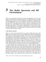
I. REVIEW OF ADC FUND AMENTALS
Since the wideband ADC is one of the fundamental components of the soft-
ware radio, this chapter begins with a revie w of rele vant results from sam-
pling theory. The analog signal to be converted must be compatible with the
capabilities of the ADC or DAC. In particular, the bandwidths and linear dy-
namic range of the two must be compatible. Figure 9-1 shows a mismatch
between an analog signal and the ADC. For uniform sampling rate
f
s
,the

maximum frequency for which the analog signal can be unambiguously re-
constructed is the Nyquist rate,
f
s
=
2. The wideband analog signal extends
beyond the Nyquist frequency in the figure. Because of th e periodicity of
the sampled spectrum, those components that extend beyond the Nyquist fre-
quency fold back into the sampled spectrum as shown in the shaded parts
of the figure (thus the term
folding frequency
). This is well known as alias-
ing [274, 275]. Although some aliasing is unavoidable, an ADC designed for
software-radios must keep the total power in the aliased components below
the minimum level that w ill not unacceptably distort the weakest s ubscriber
signal.
Figure 9-1
Aliasing distorts signals in the Nyquist passband.
289
290
ADC AND DAC TRADEOFFS
A. Dynamic Range (DNR) Budget
If acceptable distortion is defined in terms of the BER, then dynamic range
(DNR) may be set by the following procedure:
1. Set BER
THRESHOLD
from QoS considerations
2. BER =
f
(MODULATION, CIR, FEC)

3. BER
<
BER
THRESHOLD
"
CIR
>
CIR
THRESHOLD
, from
f
()
4. DNR = DNR
ADC
+DNR
RF
#
IF
+DNR
OVERSAMPLING
+DNR
ALGORITHMS
5.
P
ALIASING+RFIF+NOISE
<
1
2
(DNR
ADC

+CIR
THRESHOLD
)
Consider the situation where the channel symbol modulation, MODULA-
TION, is fixed (e.g., BPSK). BER is a function of the CIR. The first step in es-
tablishing the acceptable aliasing power is to set the BER
THRESHOLD
by consid-
ering the QoS requirements of the waveform (e.g., voice). The BER
THRESHOLD
for PCM voice is about 10
#
3
. The next step is to characterize the relationship
between BER and CIR. In the simplest case, this relationship is defined in
the BER-SNR (CIR or Eb/No) curve for MODULATION (e.g., from [275]).
In other cases, FEC reduces the net BER for a given raw BER from the mo-
dem. In such cases, net BER has to be translated into modem BER using the
properties of the FEC code(s) [276, 277]. BER
THRESHOLD
is then translated
to CIR
THRESHOLD
using
f
(e.g., 11 dB). Finally, one must incorporate the in-
stantaneous dynamic range requirements of the ADC. Total dynamic range
must be partitioned into dynamic range that the AGC, ADC, and algorithms
must supply. In the simplest case, the total dynamic range is just the near–far
ratio plus CIR

THRESHOLD
. If the RF and/or IF stages contain roofing filters or
AGCs, then some of the total system DNR is allocated to these stages. In addi-
tion, since the wideband ADC of the SDR oversamples all subscriber signals,
digital filtering can yield oversampling-gain. O ther postprocessing algorithms
such as digital interference cancellation can yield further DNR gains. Each
such source of DNR reduces the allocation to the ADC. From these relation-
ships, one establishes DNR
ADC
. The power of aliasing, spurious responses
introduced in RF and/or IF processing, and noise should be kept to less than
half of the LSB of the ADC.
If the total power is less than the power represented by
1
2
of the least sig-
nificant bit (LSB) of the ADC, then all of the A DC bits represent processable
signal power. If the power exceeds
1
2
LSB, then this extra precision presents a
computational burden that has to be justified. For example, the extra bits may
result from rounding up from a 14-bit ADC to the more convenient 16 bits
in order to transfer data efficiently. When this is done, the difference between
accuracy and precision should be kept clear.
B. Anti-Aliasing Filters
When the aliased components are below the minimum acceptable power le vel
(e.g.,
1
2

LSB) the sampled signal is a faithful representation of the analog sig-
REVIEW OF ADC FUNDAMENTALS
291
Figure 9-2
Anti-aliasing fi lters suppress aliased components.
Figure 9-3
High resolution requires high stop band attenuation.
nal, as illustrated in Figure 9-2. The wideband ADC, therefore, is preceded
by anti-aliasing filter(s) that shape the analog spectrum to avoid aliasing. This
requires anti-aliasing filters with sufficient stop-band attenuation. Figure 9-3
shows the stop-band attenuation required for a given number of bits of dy-
namic range. Since the instantaneous dynamic range cannot exceed the reso-
lution of the ADC, the number of bits of resolution is a limiting measure of
the dynamic range. High dynamic range requires high stop-band attenuation.
To reduce the power of out-of-band energy to less than
1
2
LSB, the stop-
band attenuation of the anti-aliasing filter of a 16-bit ADC must be
#
102 dB.
This includes the contributions of all cascaded filters including the final anti-
aliasing filter.
To suppress frequency components that are close to the upper band-edge
of the ADC passband, the anti-aliasing filters r equire a large shape factor.
The shape factor is the ratio of the frequency at which
#
80 dB attenuation
is achieved versus the frequency of the
#

3 dB point. Bessel filters have high
shape factors and thus slow rolloff, but they are monotonic. Monotonic fil-
ters exhibit increased attenuation as frequency increases. Nonmonotonic filters
have decreased-attenuation zones. These admit increased out-of-band energy
and distort phase. Those filters with fastest rolloff also have high amplitude
ripple and distort phase more than filters with more modest rolloff. Filter de-
sign has received much attention in the signal-processing literature [278]. (See
Figure 9-4.)
292
ADC AND DAC TRADEOFFS
Figure 9-4
Attenuation rolloff, amplitude ripple, and shape factor determine anti-
aliasing filter suitability.
Figure 9-5
Sample-and-hold circuits limit ADC performance.
C. Clipping Distortion
In most applications, one cannot control the energy level of the maximum
signal to be exactly equal to the most significant bit. One must therefore
allow for some AGC or for some peak power mismatch. Clipping of the peak
energy level introduces frequency domain sidelobes of the high power signal.
These sidelobes have the general structure of the convolution of the signal’s
sinusoidal components with the Fourier transform of a square wave, which
has the form of a sin(
x
)
=x
function. Frequency domain sidelobes have a power
level of
#
11 dB, which is clearly unacceptable interference with other signals

in a wideband passband. In practice, avoiding clipping may occupy the entire
most significant bit (MSB). Usable dynamic range may therefore be one or
two bits less than the ADCs resolution.
D. Aperture Jitter
Sample-and-hold circuits als o limit ADC performance as illustrated in Fig-
ure 9-5. Consider a sinusoidal input signal,
V
(
t
)=
A
cos(
!t
), where
!
is the
REVIEW OF ADC FUNDAMENTALS
293
maximum frequency. The rate of change of voltage is as shown, yielding
a maximum rate of change of 2
A=
(2
B
)or
A=
(2
(
B
+1)
). The time duration of

this differential interval is inversely proportional to the frequency and the
exponential of the number of bits in the ADC. This period is the aperture
uncertainty, the shortest time taken for a maximal-frequency sine wave to
traverse the LSB. The timing jitter m ust be a small fraction of the aperture
uncertainty to keep the total error to less than
1
2
LSB. Therefore, the timing
jitter should be 10% or less of the uncertainty shown in the figure. An 8-bit
ADC sampling at 50 MHz requires aperture jitter that is less than a picosecond
(ps).
This stability must be maintained for a period of time that is inversely pro-
portional to the frequency stability that one requires. If, for example, the min-
imum resolvable frequency component for the signal processing algorithms
should be 1 kHz, then the timing accuracy over a 1 ms interval should be less
than the aperture uncertainty. Short-term jitter can be controlled to less than
1 ps for 1 ms with current technology. If the spectral components should be
accurate to 1 Hz, then the stability must be maintained for 1 second. Due to
drift of timing circuits, such performance may be maintained for 10
9
to 10
11
aperture periods, or on the order of 1 to 100 ms. Stability beyond these rela-
tively short intervals is problematic due to drift induced by thermal changes,
among other things. A sampling rate of 1 GHz with 12 bits of resolution
requires about 2 fs of aperture jitter or less. This stability is beyond the cur-
rent state of the art, which corresponds to 6.5 to 8 bits of resolution at these
sampling rates.
E. Quantization and Dynamic Range
Quantization step size is related to power according to [279]:

P
q
=
q
2
=
12
R
where
q
is the quantization step size, and
R
is the input resistance. The SNR
at the output of the ADC is
SNR = 6
:
02 B + 1
:
76 + 10log(
f
s
=
2
f
max
)
where
B
is the number of bits in the ADC,
f

s
is the sampling frequency, and
f
max
is the maximum frequency component of the signal.
For Nyquist sampling,
f
s
=2
f
max
, so t he ratio of these quantities is unity.
Since the log of unity is zero, the third term of the equation for SNR above is
eliminated. The approximation for Nyquist sampling, then, is that the dynamic
range with respect to noise equals 6 times the number of bits. This equation
suggests that the SNR may be increased by increasing the sampling rate be-
yond the Nyquist rate. This is the principle behind the
sigma-delta/delta-sigma
ADC.
294
ADC AND DAC TRADEOFFS
Figure 9-6
Walden’s analysis of ADC technology.
F. Technology Limits
The relationship between ADC performance and technology parameters has
been studied in depth by Walden [280, 281]. His analysis addresses the elec-
tronic parameters, aperture jitter , thermal effects, and conversion-ambiguity .
These are related to specific devices in Figure 9-6. The physical limits of
ADCs are bounded by Heisenberg’s uncertainty principle. This core phys-
ical limit suggests that one could implement a 1 GHz ADC with 20 bits

(120 dB) of dynamic range. To accomplish this, one must overcome thermal,
aperture jitter, and conversion ambiguity limits. Thermal limits may yield to
research in Josephson Junction or high-temperature superconductivity (HTSC)
research. For example, Hypress has demonstrated a 500 Msa/sec (200 MHz)
ADC w ith dynamic range of 80 dB operating at 4K [435]. Walden notes
that advances in ADC technology have been limited. During the last eight
years, SNR has improved only 1.5 bits. Substantial investments are required
for continued progress. DARPA’s Ultracomm program, for example, funded
research to realize a 16-bit
$
100 MHz ADC by 2002 [282]. Commercial re-
search continues as well, with Analog Devices’ announcement of the AD6644,
a 14-bit
$
72 MHz ADC consuming only 1.2 W [282].
II. ADC AND DAC TRADEOFFS
The previous section characterized the Nyquist ADC. This section provides
an overview of important alternatives to the Nyquist ADC, emphasizing
ADC AND DAC TRADEOFFS
295
Figure 9-7
Oversampling ADCs leverage digital technology.
the tradeoffs for SDRs. It also includes a brief introduction to the use of
DACs.
A. Sigma-Delta (Delta-Sigma) ADCs
The sigma-delta ADC is also referred to i n the literature as the delta-sigma
ADC. The principle is understood by considering an analogous situation in
visual signal (e.g., image) processing. The spatial frequency of a signal is in-
versely proportional to its spatial dimension. A large object in a picture has
low spatial frequency while a small object has high spatial frequency. Spa-

tial dynamic range is the number of levels of grayscale. A black-and-white
image has one bit of dynamic range, 6 dB. But consider a picture in a typi-
cal newspaper. From reading distance, the eye perceives levels of grayscale,
from which shapes of objects, faces, etc. are evident. But under a magnifying
glass, typical black-and-white newsprint has no grayscale. Instead, the picture
is composed of black dots on a white background. These dots are one-bit
digitized versions of the original picture. The choice between white and black
is also called zero-crossing. The dots are placed so close together that they
oversample the image. The eye integrates across this 1-bit oversampled im-
age. It thus perceives the low-frequency objects with much higher dynamic
range than 6 dB. The gain in dynamic range is the log of the number of zero-
crossings over which the eye integrates. Zakhor and Oppenheim [283] explore
this phenomenon in detail, with applications to signal and image processing.
Thao and Vetterli [284] derive the projection filter to optimally extract max-
imum dynamic range from oversampled signals. Candy and Temes offer a
definitive text [285].
1. Principles
The fundamentals of an oversampling ADC for SDR appli-
cations are illustrated in F igure 9-7. A low-resolution ADC such as a zero-
crossing detector oversamples the signal, which is then integrated linearly. The
integrated result has greater dynamic range and smaller bandwidth than the
oversampled signal. The amount of oversampling is the ratio of the sampling
frequency of the analog input to the Nyquist frequency, shown as
k
in the
296
ADC AND DAC TRADEOFFS
figure. This follows
SNR
%

=
6 B + 10 log(
f
s
=
2
f
max
) = 6 B + 10 log(
kf
Nyquist
=
2
f
max
)
Since
f
Nyquist
=2
f
max
, the oversampling rate must be at least 2
kf
max
.With
continuous 1 :
k
integration of the zero-crossing values, the output register
contains a Nyquist approximation of the input signal.

Since the integrated output has an information bandwidth that is not more
than the Nyquist bandwidth, the integrated values may be decimated without
loss of information. Decimation is the process of selecting only a subset of
available digital samples. Uniform decimation is the selection of only one sam-
ple from the output register for every
k
samples of the undecimated stream. If
the signal bandwidth is 0.5 MHz, its Nyquist sampling rate is 1 MHz. A zero-
crossing detector with a sampling frequency of 100 MHz has an oversampling
gain of ten times the log of the oversampling ratio (100 MHz/1 MHz), 20 dB.
The single-bit digitized values may be integrated in a counter that counts up to
at least 100. Although this is the absolute minimum requirement, real signals
may exhibit DC bias. A counter with only a capacity of 100 could tolerate no
DC bias. A counter with range that is a power of two, e.g., 128, tolerates up
to log(28) bits or 4.7 of DC bias. For a range of 128, a signed binary counter
requires log
2
(128) bits or 7 bits plus a sign bit. The counter treats each zero-
crossing as a sign bit, +1 or
#
1. The decimator takes every 100th sample
of this 8-bit counter, with an output-sampling rate to 1 MHz as required for
Nyquist sampling.
Zero-crossing detectors do not work properly, however, if there are insuffi-
cient crossings to represent the signal. For example, if DC bias drifts beyond
the full-scale range of the detector, then there will be no zero-crossings and no
signal. A signal may be up-converted, amplified, and clipped to force the re-
quired zero-crossings. A similar effect can be realized in linear oversampling
ADCs through the addition of dither. A dither signal is a pseudorandomly
generated train of positive and negative analog step-functions. The dither is

added to the input of the ADC before conversion (but after anti-alias filter-
ing). The corresponding binary stream is subtracted from the oversampled
stream. Alternatively, an integrated digitized replica of the dither signal may
be subtracted from the integrated output stream. This forces zero-crossings,
enhancing the SNR. One may view dithering as a way of forcing spurs gen-
erated by sample-and-hold nonlinearities to average across multiple spectral
components, enhancing SNR.
In addition, high power out-of-band components w ill be sampled directly
by the zero-crossing detector. These components will then be integrated, sub-
ject to the bandwidth limitations imposed by the integrator-decimator. The
anti-aliasing filter therefore must control total oversampled power so that it
conforms to the criteria for Nyquist ADCs.
2. Tradeoffs
There are several advantages to oversampling ADCs. First, sam-
ple-and-hold requirements are minimized. There is no sample-and-hold
ADC AND DAC TRADEOFFS
297
circuit in a zero-crossing detector. Simple threshold logic, possibly in con-
junction with a clamping amplifier, yields the single-bit ADC.
Aperture jitter remains an issue, but the jitter is a function of the number
of b its, which is 1 at the oversampling rate. This minimizes aperture jitter
requirements for a given sample rate. As the oversampled values are integrated,
the jitter averages out. In order to support large dynamic range for narrowband
signals, the timing drift (the integration of aperture jitter) should contribute
negligibly to the frequency components of the narrowband signal. This means
that integrated jitter should be less than 10% of the inverse of the narrowband
signal’s bandwidth, for the corresponding integration time.
In addition, the anti-aliasing filter requirements of a sigma-delta ADC are
not as severe as for a Nyquist ADC. The transfer-function of the anti-aliasing
filter is convolved with the picket-fence transfer-function of the decimator.

Thus, the anti-aliasing filter’s shape factor may be 1
=k
that of a linear ADC
for equivalent performance. Many commercial products use oversampling and
decimation within an ADC chip to achieve the best combination of bandwidth
and dynamic range.
Oversampled ADCs work well if the power of the out-of-band spectral
components is low. In cell site applications, Q must be very high in the filter
that rejects adjacent band interference. Superconducting filters [286] may be
appropriate for such applications.
B. Quadrature Techniques
Nyquist ADC samples signals that are mathematically represented on the real
line. Quadrature sampling uses complex numbers to double the bandwidth
accessible with a given sampling rate.
1. Principles
Real signals may be projected onto the cosine signal of an
LO and onto the sine reference derived from the same LO. This yields an
in-phase (I) signal and a quadrature (Q) signal, an I&Q pair. The in-phase
signal is the inner product of the signal with a reference cosine, w hile the
quadrature signal is the inner product with the corresponding sine wave. In
the complex plane, the in-phase component lies on the real axis, while the
quadrature component lies on the imaginary axis. If the underlying technology
limits the clock r ate to
f
c
, then the real sampling rate is also limited to
f
c
.
The Nyquist bandwidth is limited to

f
c
=
2. On the other hand, if the signal is
projected into I&Q components, each channel may be sampled independently
at rate
f
c
. The Nyquist bandwidth is then the same as the sampling rate as
illustrated in Figure 9-8. This doubles the N yquist rate for a given maximum
ADC sampling rate.
Quadrature sampling is the simplest of the polyphase filters. The concept
may be extended to multirate filter banks [287]. These advanced techniques
include the parallel extraction of independent information streams from real
signals.
298
ADC AND DAC TRADEOFFS
Figure 9-8
In-Phase and quadrature (I&Q) conversion reduces sampling clocks.
2. Tradeoffs
Although theoretically interesting, analog implementations of
quadrature ADCs are challenging. Refer again to Figure 9-8. The modulators,
signal paths, and low-pass filters in each I&Q path must be matched exactly
in order for the resulting complex digital stream to be a faithful representation
of the input signal. Any mismatches in the amplitude or group delay o f the
filters yields distortion of complex signal.
Historically, it has been difficult to obtain more than 30 dB of fidelity from
quadrature ADCs. Military temperature ranges exacerbate the problems of
matching the analog paths. Integrated circuit paths are more readily matched
than lumped components. Short lengths of signal paths are easier to match,

as are resistors and other passive components on IC substrates. Since the
components are very close together, the thermal difference between the filters
is less than in lumped-circuit implementations. IC implementations of I&Q
ADCs can be effective.
To date, the best results for research-quality ADCs have been obtained
using real-sampling wideband ADCs in conjunction with digital quadrature
and IF filtering. This was the approach used in SPEAKeasy I, for example.
C. Bandpass Sampling (Digital Down-Conversion)
Nyquist sampling is also called low-pass sampling because the ADC recovers
all frequency components from DC up to the Nyquist frequency. Bandpass
sampling digitally down-converts a band of frequencies having the Nyquist
bandwidth but translated up in frequency by some multiple of
f
s
=
2.
1. Principles
When frequency c omponents are recovered from a Nyquist
ADC stream, the maximum recoverable frequency component is
f
s
=
2=
W
Nyquist
.
The minimum resolvable frequency is inversely proportional to the duration
of the observation interval. The observation interval is defined by the number
of time-domain points in that observation. The time-delay elements in a digital
filter constitute an observation interval. A fast Fourier transform (FFT) is an

observation interval of
N
real samples. If
N
= 1024 and
f
s
=1
:
024 MHz, then
ADC AND DAC TRADEOFFS
299
Figure 9-9
Bandpass sampling converts channels directly to baseband. (a) time do-
main; (b) frequency domain.
the minimum recoverable frequency and the resolution of each cell are both
f
s
=
1024, or 1 kHz. The FFT has a DC component that is the average value of
the signal over the observation interval
T
s
&
1024, which is 1 ms. The first
N=
2
or 512 FFT bins are not redundant. They represent the frequencies from
f
s

=N
to
f
s
=
2, 512 kHz. Thus, the low-pass nature of the Nyquist sampling process
defines frequency components from DC to
f
s
=
2.
25
The principle of bandpass sampling is to sample a passband of bandwidth
W
Nyquist
centered at frequency
kfs
(
k
'
2,
k
is even), at the Nyquist rate
fs
.
The high-frequency components are translated to baseband by the frequency-
translation property of subsampling. Figure 9-9a illustrates the subsampling
process in the time domain. The high-frequency sinusoid represents the upper
cutoff frequency of a bandpass signal, occurring at an integer multiple of
the Nyquist frequency. Sampling this frequency at the Nyquist rate creates

a beat-frequency, which translates the signal to baseband, the low-frequency
sinusoid of the figure. The frequency-domain representation (Figure 9-9b)
shows how a passband centered at 2
f
s
(circled) is translated to baseband below
f
s
=
2.
One advantage of this approach is that the subband of interest is translated
in frequency without the use of a mixer stage, and with no LO, either analog
or digital. The primary disadvantage is that all of the power in the frequency
components between the selected subband and DC are aliased into the base-
band. Therefore any residual energy in the bands centered at
kfs
is integrated
25
This analysis employs sinusoids as the basis functions used in the observation. Wavelet-basis
functions yield different observations.
300
ADC AND DAC TRADEOFFS
into the baseband. Bandpass-filtering requirements for this approach therefore
must keep the total power in the intervening bands to less than
1
2
LSB.
2. Tradeoffs
SDR RF bands generally have bandpass characteristics, not
low-pass characteristics. A cellular uplink, for example, might consist of

25 MHz from 824 to 849 MHz. The ideal software radio would convert directly
from RF at a sampling rate of say 2.3 GHz. The Nyquist frequency defines a
low-pass digital spectrum from DC to 1 GHz. Bandpass sampling of the same
cellular b and requires a bandpass sampling rate of only 2
&
25 = 50 MHz, not
2
&
849 = 1698 MHz. In terms of ADC rates, bandpass sampling presents an
attractive alternative to Nyquist sampling.
In order to translate the passband without distortion, the intervening spectra
between 3
fs=
2and5
fs=
2 must be suppressed. A high-
Q
analog bandpass
filter or cascade of filters suppresses the unwanted parts of the spectrum. Such
filters have historically not been available. Consequently, the superheterodyne
receiver translates the bandpass signal to an IF where Nyquist sampling tech-
niques suffice. High-
Q
filters such as those emerging from the MEMS program
may facilitate bandpass sampling. At present, one cannot obtain equivalent
signal quality and dynamic range from bandpass sampling as from the su-
perheterodyne receiver. Bandpass sampling will no doubt continue to attract
research and development interest [288].
D. DAC Tradeoffs
DACs convert digital signals to analog waveforms. Good DAC design incor-

porates not just level conversion but also high linearity (low intermodulation
products), integrated filtering, grounding, and isolation of the digital clock
from the analog output waveform. In addition, DACs for cell site applications
require oversampling for improved smoothness. This reduces out-of-band ar-
tifacts. The design principles of DACs are similar to ADCs. D AC setup and
hold corresponds to the sample and hold of the ADC. Setup-and-hold time
therefore determines the fidelity of signal reconstruction in a way that corre-
sponds to the effects of aperture jitter in ADCs.
Harris Corporation’s 12-bit 100 MHz DAC (HI5731) has spurious-free dy-
namic range of
#
70 to
#
85 dBc (depending on windowing and oversampling).
Its integral linearity error is 1.5 LSB. Full-scale gain error is 10% maximum
[289]. For cell site applications, this DAC will generate 12.5 to 25 MHz of
total output bandwidth. A mplifiers used in the cable TV industry have 1 GHz
output bandwidth from a few MHz to 1 GHz with flat amplitude and phase
response. Such amplifiers are appropriate for the amplification of analog IF
in cell site applications.
Phase coherence of the multiple parallel IF waveforms combined into one
DAC stream can cause the output amplifiers to saturate at peak power. There is
a 20 dB difference in peak-to-average power ratio between a single sine wave
and a base station application with 100 phase coherent IF sine waves. The
SDR APPLICATIONS
301
Figure 9-10
Sampling rate depends on the application.
random phasing of these digital signals reduces the peak-to-average power
ratio proportionally. This improves the efficiency of the amplifier and reduces

the likelihood of saturation. One should therefore assure that the RF modem
software randomizes phase to distribute output power uniformly in the time
domain. This is another example of a way in which the design of the digital
processing algorithms and hardware can yield benefits (or cause problems)
for the analog parts of the software radio.
III. SDR APPLICATIONS
ADC and DAC applications are constrained by sampling rate and dynamic
range. The pace of product insertion into wireless devices is also determined by
power dissipation. Infrastructure applications that are not power-constrained
may evolve toward digital RF. This section highlights these aspects of ADC
and DAC applications.
A. Conversion Rate, Dynamic Range, and Applications
ADC sampling rates and dynamic range requirements depend on the appli-
cation. Figure 9-10 shows how increasingly wideband applications require
increasingly large instantaneous dynamic range. Analog filtering an d AGC
achieve 90 to 100 dB or more of total dynamic range. As one increases the
instantaneous bandwidth, one must also increase the instantaneous DNR as
shown in Figure 9-10. It differentiates baseband (BB), IF, and RF ADC re-
quirements. Baseband refers to the bandwidth of modulation of a single RF
302
ADC AND DAC TRADEOFFS
Figure 9-11
Present ADCs offer viable applications.
carrier. Thus, HF baseband consists of typically 5 Hz to 3 kHz of modulated
RF carrier. HF automatic link establishment (ALE) may employ linear FM
(chirp) waveforms that use more bandwidth, increasing sampling rate require-
ments accordingly. Voice channel modems and music require only a few tens
of kHz of bandwidth, but with appreciable DNR for high fidelity applications.
Baseband ADC is the technology of classical programmable digital radios.
Frequency division multiplexed (FDM) signals have a few MHz IF-band-

width, while PCM, cellular band allocations, 3G, and air navigation signals
require tens of MHz. IF-ADC is the technology of SDR. Miller [290] derives
the RF DNR requirements of HF as 120 dB, consistent with [291]. CDMA
bands are not as demanding of DNR because they are power managed. The
RF-ADC is the technology of the ideal software radio. As the bandwidth
increases from BB to IF to RF, the instantaneous DNR increases by about
30 dB per change.
B. ADC Product Evolution
Figure 9-11 shows the relationship of commercially available ADC perfor-
mance to research devices, emerging technology, and maximum requirements
from Figure 9-10. Many viable SDR applications are workable with currently
available technology. Fielded applications include baseband digital signal pro-
cessing in programmable digital radios. Emerging applications include SDRs
that use IF conversion and parallel ADC channels to obtain high dynamic
range. SPEAKeasy I and II, for example, both employed IF conversion with
moderate (1 MHz) and wideband (70 MHz) ADC channels. The dynamic
SDR APPLICATIONS
303
Figure 9-12
Low-power ADCs driven by wireless marketplace.
range of these implementations did not fully address the maximum require-
ments for radio applications. But they established the feasibility of the tech-
nology, allowing developers to gain experience with SDR architecture.
C. Low-Power Wir eless Applications
The recent evolution of ADC product has been driven significantly by the
wireless marketplace. Handheld commercial audio devices motivate invest-
ment in devices with less than 1 MHz sampling rates but more than 100 dB
SNR. Wireless handset applications provide much of the impetus behind low-
power wideband ADC chips. Figure 9-12 shows the difference in sampling
rate and dynamic range between low-power ADCs and ADCs for board-level

products (e.g., for research and laboratory instrumentation markets). The 10-
and 12-bit 70 MHz ADCs are rapidly evolving to 14-bit products.
D. Digital RF
As ADCs continue to evolve, they will enable the digital RF architecture illus-
trated in Figure 9-13. Traditional RF subsystems include preamplifiers, LNAs,
filters, RF distribution, and frequency translation and filtering stages that trans-
late RF to usable IF signals. Such RF subsystems may comprise upward of
60% of the manufacturing cost of a radio node. These subsystems require
large amounts of expensive touch-labor to assemble waveguide, coaxial cable,
304
ADC AND DAC TRADEOFFS
Figure 9-13
Digital RF replaces analog waveguide/coax with digital fiber.
Figure 9-14
Digital RF could provide 80 dB of dynamic range.
Figure 9-15
High-performance ADCs have been demonstrated.
and other discrete components. The digital RF alternative, also shown in Fig-
ure 9-13, uses a preamplified ADC and multiplexer at the antenna to create a
Gbps fiber optic signal [292]. Digital RF distribution via gigabit fiber optics
weighs less and costs less per meter than RF distribution via coax or waveg-
uide. In addition, fiber optics costs less to install and maintain than coax and
waveguide. Lack of dynamic range, digital-RF’s major shortfall at this time,
can be enhanced using digital filtering techniques.
To see this, consider the use of a 6 GHz ADC [280] as illustrated in Figure
9-14. Although the RF ADC has a limited dynamic range, its high sampling
rate oversamples the bandpass bandwidth of an AMPS signal. The oversam-
pling gain increases the dynamic range through integrating digital filters as
discussed above. The 25 MHz bandwidth of the cell site is 21 dB less than the
RF sampling rate, yielding 51 dB of dynamic range within the cellular band.

The subscriber bandwidth of 30 kHz offers an additional 29 dB of gain, yield-
ing an aggregate DNR of 80 dB. Thus, the power in the digitally integrated
baseband signals may range linearly over 80 dB. This results from the 30 dB
of DNR at RF and the integrating digital filters that follow. Figure 9-15 shows
some recent high-performance ADC products with sponsor or manufacturer.
Any of the products with 2, 3, 4, and 6 GHz sampling rates could be the
ADC DESIGN RULES
305
Figure 9-16
Nonlinearities characterized by compression and intercept points.
basis for digital RF. The Hypress supercooled ADC may accelerate progress
towards digital RF [435].
IV. ADC DESIGN R U LES
The ADC determines the quality of the digital signal available for subsequent
digital signal processing. The parameters that most shape SDR applications are
linearity and dynamic range. Dynamic range can be established empirically
by the measurement of SNR. Several methods are available for making such
measurements, and some are more relevant to SDR than others. Such measure-
ments allow one to establish SNR and DNR budgets from the antenna through
the product delivered to the user by matching SNR at each SDR interface. In
addition to the related design rules, the parallelism of ADCs and DACs has a
first-order impact on SDR architecture. This section provides an overview of
these technical issues and the associated design rules.
A. Linearity
ADCs exhibit nonlinear behavior characterized by the compression and inter-
cept points illustrated in Figure 9-16. Just like a mixer stage in a receiver, as
the input power is increased, the signal output power increases. It reaches the
output noise floor at a level defined by the equivalent thermal noise tempera-
ture of the device. Continued increase in the input power yields a continued
increase in the output power of the fundamental.

The point at which the power of the third-order intermodulation product of
the ADC is tangential to the output noise level determines the spurious-free
dynamic range of the ADC. As the third-order product increases, its power
eventually intersects the fundamental. This point is called the input-referenced
306
ADC AND DAC TRADEOFFS
Figure 9-17
ADC specifications depend on applications.
third-order intercept point (IP3). The output power of the fundamental satu-
rates w ell before IP3, however. The point at which the output power of the
fundamental differs from the ideal output power by 1 dB is the 1dB compres-
sion point. If two tones are present in the input, the spurious-free dynamic
range (SFDR) is termed the two-tone SFDR (2-SFDR). The maximum two-
tone spur may appear when the tones are separated by an amount that is a
harmonic of the sampling rate, for example. Generally, it is difficult to predict
the combination of tones that yields the maximum spur. The search for tone
combinations is combinatorially explosi ve. Therefore, it is important that the
ADC supplier characterize the two-tone spurious-free dynamic range at crit-
ical points, including integer multiples and halftones of the sampling rates.
Tone separations at integer multiples and harmonics should also be tested.
B. Measuring SNR
In addition to SFDR and 2-SFDR, SNR measurements are useful in specify-
ing ADC performance. The SNR of an ADC is the ratio of signal power to
nonsignal power. Nonsignal power includes thermal noise and other residual
errors of the converter (Figure 9-17). This metric is most appropriate when the
bandwidth of the signal of interest is approximately the Nyquist bandwidth of
the ADC. Radar-matched filtering exemplifies such applications. Radar pulses
are typically wideband square waves. The matched-filter receiver is optimal for
the square wave when the bandwidth of the receiver is the Nyquist bandwidth
of the ADC.

The SFDR is a more appropriate metric when the bandwidth of the signal of
interest is much less than the Nyquist bandwidth of the ADC. First-generation
cellular base stations exemplify this situation. A 30 kHz AMPS carrier is
more than two orders of magnitude smaller in bandwidth than the 12.5 MHz
ADC DESIGN RULES
307
spectrum-allocation accessed by a cell-site ADC. The seven-cell f requency
reuse pattern of first-generation systems reduces the maximum density of nar-
rowband signals to 1 : 7, not considering interference from adjacent sites.
GSM’s 1 : 3 frequency reuse pattern is also well characterized by SFDR.
The density of narrowband carriers may be high, as in an analog FM-FDM
with 100% channel occupancy or CDMA, with 1 : 1 frequency reuse. In such
cases, the noise power ratio (NPR) is a more appropriate metric. The NPR is
the ratio of the spectral density outside of a notch filter to the maximum spec-
tral density inside the notch filter. The measurement is taken when the Nyquist
bandwidth is flooded with white noise. The notch filter must be deeper than
the noise power inside the notch so that the measurement defines the leakage
that the ADC causes from the adjacent channels into the channel of interest.
By sweeping the notch filter across the band, the point of maximum spectral
density inside the notch is readily identified. When all but one channel are oc-
cupied, the total power that leaks into a single unoccupied channel defines the
dynamic range available to the unoccupied channel. In addition, the full-power
analog input bandwidth is relevant to bandpass sampling. Since bandpass sam-
pling converts signals directly to baseband, the full-power bandwidth specifies
the maximum RF spectrum that may be thus converted.
C. Noise Floor Matching
One approach to the allocation of SNR and DNR through an SDR is to match
the radio noise floor to the ADC input noise level. The noise power from a
noise-limited receiver may be matched to the power of the ADCs LSB using
[279]:

P
m
=
#
174 dBm + 10 log(
W
a
)+NF
where
P
m
is the noise power of a noise limited receiver,
#
174 dBm is
kT
o
B
, Boltzmann’s constant, temperature, and unit bandwidth,
W
a
is the receiver (access) bandwidth in Hz, and
NF is the receiver noise figure in dB.
This creates a design rule that total system noise should be less than
1
2
LSB.
This rule applies to
kTB
bands in upper UHF and SHF.
ADC error noise should always be less than

1
2
LSB, but receiver noise need
not be so matched. At first, it appears inefficient to sample noise power with
many bits. But in the HF bands, for example, the noise consists of the additive
effects of large numbers of distant emitters and natural phenomena (e.g., light-
ning strikes). Consequently, the differentiation of noise from subscriber signal
depends on differentiating impulsive noise from a subscriber signal such as
an HF-ALE probe. Since the noise background may shift by 10 dB in a few
milliseconds at HF, the allocation of 2 or 3 bits of ADC dynamic range to
308
ADC AND DAC TRADEOFFS
Figure 9-18
SPEAKeasy I ADC study–defined figure of merit.
noise characterization may be appropriate. In interference-limited bands, one
may apply many bits of ADC DNR to the characterization of the interference.
This technique allows one to apply algorithms that subtract an idealized replica
of the demodulated interferer from the passband, enhancing the subscriber’s
CIR. An appropriate formulation of a design rule for ADC DNR is to allocate
sufficient bits to the noise or interference to support the needs of the CIR
enhancement algorithms.
D. Figure of Merit
A figure of merit that characterizes the level of ADC technology is the product
of sampling rate times the full-scale SFDR as summarized in Figure 9-18.
“Net” SFDR reduces full-scale SFDR by 2 bits or about 10 dB. One bit assures
that the noise power is less than
1
2
LSB. The other bit a ssures that there is
sufficient dynamic range for the input AGC to avoid saturation.

SPEAKeasy I sought to access from 2 MHz to 2 GHz in a single RF chan-
nel with a single ADC. This feat would require an ADC with at least a 5 GHz
sampling rate and 19 bits of SFDR for a total figure of merit of
#
210 dBc/Hz.
Contemporary ADCs reach the values shown in Figure 9-18. The widest prac-
tical bandwidth for SDR applications is about 65 Msps (25 MHz) at 12 to 14
bits of SFDR (72 to 84 dB full scale or about 74 dB net). This performance
is marginal for cell site applications.
E. Technology Insertion
ADCs shape the SDR architecture. In the handset, there may be no ADC
because the extremely low-power budgets drive one away from the high
dissipated-power of wideband ADCs. The lower total power of direct conver-
sion receivers is more appropriate. The nonlinear aspects of direct conversion
ADC DESIGN RULES
309
Figure 9-19
ADC technology insertion issues.
receivers do not degrade the reception of the single channel-per-band of a
handset.
In base station and mobile-node designs where large numbers of subscribers
are supported digitally, the power dissipation of a wideband ADC is accept-
able. The technical advantages of the wideband ADC-based IF architecture
then apply. Oversampling may be appropriate to enhance the effectiveness of
multiple-access interference-cancellation algorithms.
Once the ADC sampling rate is established, one may employ either real
or complex sampling. In many cases, the ADC may employ oversampling to
enhance dynamic range (e.g., sigma-delta ADC). ADC technology continues
to advance, dri ven by wireless and radar markets.
Figure 9-19 summarizes performance issues for ADC applications. SDR

technology has the potential to reduce the cost and complexity of first-genera-
tion mobile cellular base stations. One approach is to reduce the number of
analog IF and baseband channels to one, from the maximum number of ac-
tive subscribers (e.g., approximately 100). Alternatively, a dual-mode cell site
capable of both GSM and first-generation standards could have five parallel
5 MHz digital channels instead of the twenty-five 200 kHz channels of a con-
ventional G SM cell site. ADCs supporting this approach require 80 to 90 dB
of SFDR. As the cellular standards migrate from single-subscriber-per-carrier
to TDMA and CDMA, the density of occupancy of the wider-bandwidth RF
carriers increases. In order to support 3G deployment with an SDR architec-
ture, one requires an ADC capable of supporting the despreading of 20 MHz
W-CDMA channels.
This alternative is unlikely to gain wide commercial acceptance due to the
computationally intensive nature of digital despreading. A more reasonable
310
ADC AND DAC TRADEOFFS
alternative w ould be to add additional circuits to a W-CDMA rake receiver that
permits it to digitize GSM carriers. The 2G waveform may then be processed
using the 3G baseband DSP. This would be a dual-mode despreader-digitizer
chip. Such chips might also be used in military applications to despread wide-
band waveforms, and to extract narrowband waveforms for SDR processing.
F. Architecture Implications
The system DNR must be sustained from antenna through the information
stream delivered to the wireline network. Consequently, the software-radio
systems engineer must allocate DNR to RF conversion, ADC, and digital fil-
tering to maintain the required system DNR. RF conversion, in particular , may
employ AGC, which increases total dynamic range. If AGCs are incorporated
in RF, ADC, digital filtering, and demodulation, then the interactions among
these stages is complex. Consequently, SDR architecture should include facil-
ities for the allocation and management of DNR.

V. EXERCISES
1.
Does the conversion of an RF signal to digital form require the use of an
ADC? If not, what are the alternative ways of obtaining a digital represen-
tation of the RF signal?
2.
Define uniform sampling. Define Nyquist sampling. Define aliasing.
3.
What QoS metric should one use to determine anti-aliasing requirements?
(e.g., time delay? cell loss rate? other?)
4.
Differentiate among the Nyquist ADC, the sigma-delta ADC, and the quad-
rature ADC. What are the advantage(s) of the latter two over the Nyquist
ADC?
5.
Consider the disaster-relief scenario. What ADCs are applicable to opera-
tion with police and rescue aircraft in the 108 to 400 MHz b and? What is
the sampling rate of an ideal ADC to access this entire band at once? What
are the performance ramifications of implementing a system using an ADC
with this data rate? (Hint: How much dynamic range can be provided to a
25 kHz narrowband user?) What alternative ADC approaches are possible?
How will they effect the cost of the system?
6.
Considering the situation of question 5, what operational constraints could
be imposed on users of legacy radios in this band to operate with the
disaster-relief system? How can this reduce the requirements on the overall
ADC suite?
7.
How much has ADC technology improved in the last eight years? What are
the purely theoretical limits of ADC technology? W hat three technologi-

cal features of ADC technology now limit progress toward the theoretical
limits? How much should the technology improve over the next five years?
EXERCISES
311
8.
Recall the object-oriented approach to architecture analysis. Define an in-
heritance hierarchy for digital processing including ADCs, ASICs, FPGAs,
DSPs, and GP processors. What slots are needed on the ADC object class?
What criteria apply to selecting such slots? Differentiate slots needed for
an industry-standard open architecture from an enterprise-oriented archi-
tecture intended to reflect proprietary product plans.