Điện thoại di động vô tuyến điện - Tuyên truyền Channel P8 pptx
Bạn đang xem bản rút gọn của tài liệu. Xem và tải ngay bản đầy đủ của tài liệu tại đây (384.22 KB, 42 trang )
Chapter 8
Sounding, Sampling and Simulation
8.1 CHANNEL SOUNDING
In the earlier chapters we discussed the characteristics of mobile radio channels in
some detail. It emerged that there are certain parameters which provide an adequate
description of the channel and it remains now to describe measuring equipment
(channel sounders) that can be used to obtain experimental data from which these
parameters can be derived. It is often of interest to make measurements which shed
some light on the propagation mechanisms that exist in the radio channel but
engineers are usually more interested in obtaining parameters that can be used to
predict the performance, or the performance limits, of communication systems
intended to operate in the channel.
The choice of channel sounding technique will usually depend on the application
foreseen for the propagation data. Basically, a choice has to be made between using
narrowband or wideband transmissions and whether a time or frequency domain
characterisation is required. In what follows we will brie¯y describe both
narrowband and wideband systems and provide an indication of how relevant
data can be extracted from measurements. We make only a brief reference to the
data processing techniques, particularly in the case of wideband channels; for details
the interested reader will need to consult the literature [1±4].
8.2 NARROWBAND CHANNEL SOUNDING
It is clear from the earlier discussion that when the mobile radio channel is excited by
an unmodulated CW carrier (i.e. a single tone), large variations are observed in the
amplitude and phase of the signal received by a moving antenna. These variations
are apparent over quite small distances. A considerable number of mobile radio
propagation studies have been undertaken by transmitting an unmodulated carrier
from a ®xed base station, receiving the signal in a moving vehicle and recording the
signal envelope. It is common to use a receiver which provides a DC output voltage
proportional to the logarithm of the received signal amplitude, and a suitable
receiver calibration therefore produces the signal strength in dBm or, if a calibrated
antenna is used, the ®eld strength in dBmV/m.
Figure 8.1 shows a simpli®ed block diagram of a generic receiving and recording
system which has the basic features required. The signal envelope at the output of the
The Mobile Radio Propagation Channel. Second Edition. J. D. Parsons
Copyright & 2000 John Wiley & Sons Ltd
Print ISBN 0-471-98857-X Online ISBN 0-470-84152-4
receiver is fed via a suitable interfacing circuit and an ADC into the memory (RAM)
of a microcomputer. Distance pulses from a transducer are used to trigger the ADC
so that samples are taken at an appropriate rate. Analysis of the stored data can
either be carried out in suitable batches as ®eld trials proceed or the stored data can
be retained for analysis later. It is not always convenient, or necessary, to initiate
sampling using distance pulses and if the system is made portable for use within a
room or building, for example, then time sampling is much more convenient.
The phase of the received signal is sometimes of interest and can be measured,
relative to a ®xed reference, if the signal is demodulated in two quadrature channels.
Such receivers have been used by Bultitude [5] for indoor measurements and by
Feeney [6] for small-cell measurements outdoors. To measure phase accurately it is
essential that the local oscillators in the transmitter and receiver are phase-locked. In
the majority of cases this is impracticable but the use of extremely stable sources,
such as rubidium oscillators, can provide adequate coherence over quite long periods
of time. In this manner, only those phase variations introduced by the propagation
channel, and not those due to the transmitter/receiver combination, are measured.
Of course, the phase information cannot realistically be studied at the carrier
frequency. Translation of the quadrature information to a suitable lower frequency
can be carried out by heterodyning to an intermediate frequency; two possibilities
exist, either a conveniently low intermediate frequency or a direct conversion to zero-IF.
In the ®rst type of receiver, care is needed in the choice of IF to avoid images,
arising from the mixing process, from falling within the passband of the IF ®lter.
This can be achieved using an initial frequency upconversion or by employing image
rejection mixers. Two advantages exist for this architecture: the input frequency is
not restricted to a narrow RF band and a suitable network analyser can be used to
isolate sources of amplitude and phase unbalance in the various signal paths. The
zero-IF (direct conversion) receiver requires mixers which have a suciently high
operating frequency at the RF port, together with a DC-operating IF port. The
operating frequency is restricted to a narrow range due to the constraint of
maintaining quadrature in the various signal paths. High RF power levels are
required to drive the mixers, so that an adequate dynamic range is achieved.
These disadvantages are minimised if the design is limited to one carrier frequency.
Other advantages also exist; for example, only one phase-locked stage is required
222 The Mobile Radio Propagation Channel
Figure 8.1 Simpli®ed block diagram of a receiver and data logging system for use in the ®eld.
and the single mixing process down to zero-IF provides an inherent detection
function. Images are no longer a problem because they are well separated from the
wanted information and are easily removed. Any imbalance in the amplitude or
phase responses of the two channels can be reduced or eliminated through careful
calibration or the use of digital correction techniques. Figure 8.2 shows the dual-
channel receiver used by Feeney [6] for propagation and diversity experiments at
900 MHz. A dynamic range of 45 dB was achieved.
8.2.1 A practical narrowband channel sounder
For characterising the channel in respect of its likely eect on narrowband systems it
is usually adequate to transmit a CW carrier and to measure the variation in the
envelope as the receiver is moved around within a given small area. Almost without
exception, equipment designed for this purpose uses a ®xed transmitter and a mobile
receiver. A data acquisition and analysis unit can easily be incorporated into the
receiving system and designs can be tailored to meet any speci®c requirement, e.g.
outdoors or indoors, or in con®ned spaces. The equipment described below was used
by Davies [7] for indoor measurements but it is not restricted in any way and could
easily ®nd other applications.
A backpack system was preferred so that the operator could move around freely.
This necessitated battery operation with a battery capacity adequate for several
hours of operation. The system was speci®ed to have a dynamic range of 80 dB at
1.8 GHz, an automated attenuation control to allow the operator to walk into a
room or area and conduct a test without any pretesting routine and a data
acquisition system which stored not only the samples of signal strength, but also the
setting of the attenuator control. Time sampling was used, the sampling rate being
such that 4 or 5 samples per wavelength were taken at normal walking speed. The
data acquisition system was designed to enable a large number of samples to be
taken, subsequently averaged and the mean value stored.
Sounding, Sampling and Simulation 223
Figure 8.2 Feeney's dual-branch, phase-locked direct conversion receiver.
It was also designed to acquire the average signal level and CDF for a large number of
locations. It was intended that the signal strength data should be analysed using a
notebook computer, accessed via its printer port. Since it is not possible to insert a
standard data acquisition card into such a computer, and since access via the printer port
interface is slow, it was necessary for the data acquisition system to have on-board
memory so that signal could be sampled and stored for downloading later. The notebook
computer eectively controls the acquisition via a specially written program, and allows
downloading from the on-board memory to the hard disk for permanent storage.
The transmitter was of conventional design; it used a commercial frequency
synthesiser as a signal source, the output being ampli®ed to provide an output power of
3 W, before being fed to a 5l/16 collinear antenna. A simpli®ed block diagram of the
receiver, which is based on a single-conversion superheterodyne architecture, is shown
in Figure 8.3. The receiving system is in two parts, a backpack unit and a handset
similar in size to a modern cellphone, which incorporates the receiving antenna.
In the receiver, the signal passes through an RF ampli®er and bandpass ®lter
before being downconverted to a 10 MHz IF. Further ®ltering is provided by a
crystal ®lter with very sharp roll-o characteristics and the signal is then fed to a
logarithmic IF ampli®er/detector which has a dynamic range in excess of 80 dB. The
input range of the receiver is controlled by the use of a programmable attenuator
having a range of 128 dB in 1 dB steps. The control of this attenuator is automatic
via the logging system and its setting is stored.
The ecient logging of data is carried out by the data acquisition unit (DAU).
Since it is only required that the mean signal level be recorded, a system was designed
to enable the output of the receiver to be sampled and averaged in batches to produce
a single value. A diagram of the DAU system is shown in Figure 8.4. The computer
interface allows any recorded data to be downloaded to an IBM-compatible
computer and stored for later analysis. If it is desired to have approximately 4±5
samples per wavelength at an average walking speed of 1.5 m/s, then the sampling
frequency required is approximately 40 Hz at 1800 MHz (l % 17 cm).
The microprocessor used for this application is the Texas Instruments TMS320-E15.
This processor has the advantage that its program memory is contained in the on-chip
EPROM of the device, so reprogramming is straightforward. The processor interfaces
with several devices, namely an analogue-to-digital converter (ADC), a dynamic RAM,
the programmable attenuator and a set of input switches and LCD display located in
the handset. Interfacing with a notebook computer is performed by a parallel printer
interface on the PC. The DAU can be in one of two modes, download or record.
In record mode, the system `hangs' until the user wishes to sample. After initiating
a measurement, 128 sample values are taken via the ADC at a sampling frequency of
approximately 40 Hz. These 128 values are averaged to produce the mean signal level
and if necessary an adjustment is made to the programmable attenuator. The change
in attenuation is calculated automatically, using an algorithm which evaluates the
mean signal strength, the dynamic range of the system and the current attenuation
setting. A further 1024 samples are then taken at the constant sampling rate and the
mean signal strength is calculated. Signal levels for the CDF of the collected data are
also produced at probabilities of 1%, 50% and 99%. The calculated values are all
displayed on the LCD and stored in the dynamic RAM, which also features a small
backup battery to enable short-term storage of captured data.
224 The Mobile Radio Propagation Channel
Sounding, Sampling and Simulation 225
Figure 8.3 Block diagram of the receiver.
In download (or interface) mode, the user is allowed to interface the system with a
computer or manually view the contents of the memory via the LCD on the handset.
Using specially written software, full system calibration can also be undertaken. The
software also provides testing of all the DAU elements; a useful feature which can be
used before any ®eld measurements.
The power source for the backpack signal strength measuring system is provided
by a set of nickel±cadmium (NiCd) cells, producing an output voltage of
approximately 13 volts. The total current consumption of the backpack is
approximately 0.8 amps, so the battery pack will sustain the backpack for a
period of up to 7 hours of continuous use. DC±DC converters are used to provide
constant output voltages regardless of the ¯uctuations of the input power source.
The complete receiver system including DAU is shown in Figure 8.5; it has a
dynamic range of 80 dB and the noise ¯oor is at 7125 dBm.
8.3 SIGNAL SAMPLING
Any record of signal strength has to be analysed in order to obtain the required
parameters. The raw information, whether in linear or logarithmic units, has two
components which represent the slow and fast fading; the mean value is in¯uenced
by the distance from the transmitter. The analysis can be designed to obtain the
mean or median value in a certain area and/or to derive information about the ®rst-
and second-order statistics of the fading envelope.
If it is desired to obtain information about the depth and duration of fades, it is
necessary to sample the signal at a rate appropriate to the task. Expressions for the
average level crossing rate and average fade duration of a Rayleigh fading signal
have been obtained in eqns (5.43) and (5.47), and Table 5.1 gives values, in
226 The Mobile Radio Propagation Channel
Figure 8.4 The data acquisition unit.
wavelengths, with respect to the median value. For example, the average duration of
a fade 30 dB below the median value is 0.01l, and at 900 MHz this value corresponds
to a distance of 0.33 cm. Fairly rapid spatial sampling is therefore necessary to ensure
such fades are not missed. In practice there is lognormal fading superimposed on the
Rayleigh fading, and in order for results to be compared with theory it is necessary
to separate the two fading processes by a technique of normalisation.
Clarke's suggestion [8] of normalisation as a method of dealing with a signal in which
the underlying process is Rayleigh was discussed in Chapter 5. It has become widely
known as the running mean or moving average technique. The result is a new PDF
p
n
r
n
2r
n
exp Àr
2
n
whichisaRayleighprocesswiths
2
0:5 and an RMS value of unity. The question now
arises as to what is a suitable distance for normalisation of experimental data? Parsons
and Ibrahim [9] experimented with various windows having widths between 2l and 64l,
coming to the conclusion that it was reasonable to treat the data as a stationary Rayleigh
process for distances up to about 40 m at VHF and about 20 m at UHF. Davis and
Bognor [10] investigated the eect of measurement length on the statistics of the
estimated fast fading at 500 MHz and showed that as the distance was increased above
about 25 m, variations in the local average values appeared. It seems therefore, from
experimental evidence, that distances of up to 40 m are suitable at VHF, while there is
danger in going above 25m at UHF. We have seen that rapid sampling is necessary to
accurately obtain the second-order statistics of the signal; but following on from the
above argument we might ask, in the context of extracting the local mean value, how
many samples do we really need within the given measurement length and also, given
those samples, with what accuracy and con®dence can we estimate the local mean?
8.4 SAMPLED DISTRIBUTIONS
To answer the question about estimation of the local mean, we need to obtain some
simple relationships that apply to sampled distributions. We can state quite generally
Sounding, Sampling and Simulation 227
Figure 8.5 The complete receiving system.
that if the probability density function of a random variable x is p(x) and if x
1
,
x
2
, , x
N
are observed sample values of x, then any quantity derived from these
samples will also be a random variable. For example, the mean value of x
i
can be
expressed as
x
1
N
X
N
i1
x
i
and this is an estimate of the true mean value Efxg;
x is a random variable and the
probability density function p
1
(
x), which can be found provided p(x) is known, is
called the sampled distribution.
Generally the mean and variance of the sampled distribution can be written
^
m Ef
xgE
1
N
X
N
i1
x
i
()
1
N
E
X
N
i1
x
i
()
Efx
i
gm
8:1
and, assuming independent samples,
^
s
2
Ef
x À
^
m
2
gEf
x À m
2
g
E
1
N
X
N
i1
x
i
À m
!
2
8
<
:
9
=
;
1
N
Efx
i
À m
2
g
s
2
N
8:2
8.4.1 Sampling to obtain the local mean value
Theoretical analyses have been published that deal with the question of signal
sampling. Early work in this ®eld includes that of Peritsky [11] and Lee [12]. Peritsky
investigated the statistical estimation of the local mean power assuming independent
Rayleigh-distributed samples, and Lee presented an analysis concerned with
estimating the local mean power using an averaging process with a lowpass ®lter.
Their work was based on a statistical estimation of the RMS and mean signal
strength in volts, i.e. they assumed a receiver with a linear response. Practical
measurements, however, are often taken using a receiver with a logarithmic response;
then the signal samples are expressed directly in decibels relative to some reference
value and estimates can be made directly from them. If we consider the case of a
Rayleigh fading signal, it is possible to determine the number of independent samples
N necessary to estimate the mean or median value within a certain con®dence
interval. The need for independent samples then enables us to relate N to the distance
(length of travel) over which these samples should be obtained.
Increasing the sample size can make the estimate more accurate through a
knowledge of the eects that sampling rate and measurement length have on the
standard deviation of the estimate, but some care is needed. Simply increasing the
number of samples is not sucient since for a small measurement length they will not
be independent and may be on an unrepresentative portion of the fading envelope.
228 The Mobile Radio Propagation Channel
Similarly, a long measurement length and a sampling rate that is insucient to
resolve the fading envelope would not adequately represent the local mean or
median. It is necessary to have a suciently large sample size, and it is also necessary
to take the samples over a measurement length that allows an accurate estimation of
the required parameters.
Additionally, in the real fading environment, slow fading also exists and this will
have an in¯uence if the measurement distance is too large. It is necessary to take this
into account in order to arrive at a compromise between measurement length and
accuracy in practical measurements.
8.4.2 Sampling a Rayleigh-distributed variable
The relationships between linear and logarithmic samples of a Rayleigh-distributed
variable are derived in Appendix B. A widely used parameter is the median value r
M
of the logarithm of the signal strength. This can be obtained using (2k + 1) samples
and ®nding the sample above and below which there are exactly k samples.
Alternatively, the mean value of the logarithm of the signal strength can be found.
This is given by the mean of the dB-record:
Efr
dB
g
1
N
X
N
i1
20 log
10
r 8:3
Note that Efr
dB
g depends on the values of all the samples of r. The relationship
between this value and the value obtained from the mean of a linear receiver, i.e.
Efrg, will be related through the statistics of the signal envelope (Rayleigh in this
case) and in general this relationship will not be simple. This is not so for the median
value, which is the same sample irrespective of whether the receiver response is
logarithmic or linear. The median is widely used in mobile communications, ®rstly
because it does not require a receiver with a characteristic that closely follows a
predetermined law (say logarithmic or linear), merely one which can be calibrated
with respect to any given reading. Secondly, the 50% cumulative distribution level is
meaningful in estimating the quality of service in a given area.
8.5 MEAN SIGNAL STRENGTH
For estimation of mean signal strength in decibels, the distribution of the estimate is
not known. The estimate is obtained from the sum of independent samples, and if the
number of samples is suciently large, the distribution can be approximated by a
Gaussian distribution, using the central limit theorem, irrespective of the distribution
of the individual samples.
Let us write a standardised variable z, corresponding to a Gaussian variable x as
z
x À m
s
The probability that z is less than a speci®ed value Z is then
probz4ZPZ
Z
ÀI
1
2p
p
exp À
z
2
2
dz 8:4
P(Z) can be determined by reference to tables.
Sounding, Sampling and Simulation 229
Now, in terms of the mean signal strength that we are trying to estimate,
z
x À
^
m
^
s
which, using eqns. (8.1) and (8.2), can be written as
z
x À m
s=
N
p
8:5
Substituting this in eqn (8.4) we obtain
PZprob
x4
Zs
N
p
m
8:6
8.5.1 Con®dence interval
We are seeking to establish the number of signal strength samples, N, that are
necessary in order that we can assert, with a given degree of certainty (often
expressed as a percentage), that the mean value of these samples lies within a given
range of the true mean. This range is called the con®dence interval and can be found
by con®rming that
probÀZ
1
4z4 Z
1
Z
1
ÀZ
1
pzdz 2PZ
1
We can now extend eqn. (8.6) to obtain
prob
x À
Z
1
s
N
p
4m4
x
Z
1
s
N
p
2PZ
1
8:7
or alternatively
prob À
Z
1
s
N
p
4m À
x4
Z
1
s
N
p
2PZ
1
8:8
Table 8.1 has been compiled using Gaussian statistics and shows the range, in terms
of s, within which a given percentage of values fall. For example, 68% of values fall
within Æs.
If we are dealing with samples taken from a receiver with a logarithmic
characteristic then we know, from the relationships given in Appendix B, that
230 The Mobile Radio Propagation Channel
Table 8.1 Values of P (Z
1
) and con®dence intervals
P (Z
1
) Range
68% Æs
80% Æ1:28s
90% Æ1:65s
95.46% Æ2s
99% Æ2:58s
s 5:57 dB. Thus, 5:57=
N
p
is the standard deviation of the sample average of N
independent logarithmic samples. If we are interested in estimating within Æ1dB
then (m À
x) 1 and for 90% con®dence Z
1
is given by Table 8.1 as 1.65. Thus the
number of independent samples required is obtained from
Z
1
s
N
p
1
1:65 Â 5:57
N
p
so N 85
This is dierent from the number given by Lee [12].
If the samples are taken from a receiver with a linear characteristic then the mean
and standard deviation are related to s by eqns (5.21) and (5.23). Equation (8.8) still
applies, but s
r
is now given by (5.23). Again, the mean value is approximately
normally distributed and the sample size required to estimate within 2 dB (Æ1 dB)
with a 90% degree of con®dence is given by
20 log
10
m
r
1:65
^
s
r
À20 logm
r
À 1:65
^
s
r
52
which yields N 57. So the required sample size is greater when a logarithmic
estimator is used.
It is now necessary to relate these sample numbers to the measurement distances
over which they need to be taken. Assuming that, at the mobile, incoming multipath
waves arrive from all spatial angles with equal probability, the correlation between
the envelopes of signals measured a distance d apart is given by J
2
0
2pd=l, and for
two adjacent samples to be uncorrelated this gives d 0.38l. The minimum
distances required are therefore approximately 33l and 22l for logarithmic and
linear sampling, respectively.
Figure 8.6 is an example which shows the 95% con®dence interval for the
estimation of mean signal strength in decibels. The required sample size clearly
Sounding, Sampling and Simulation 231
Figure 8.6 Relationship between 95% con®dence interval and sample size for estimating
mean signal strength (dB) in a Rayleigh fading environment.
depends on how accurately we wish to estimate the local mean. Since the con®dence
interval decreases very slowly for large N, a smaller con®dence interval necessitates a
very much larger number of samples and a correspondingly larger measurement
distance. If the mobile is close to the base station or is in a radial street where a
strong direct path exists, the fading may be Rician rather than Rayleigh and a
smaller sample size may then be sucient. On the other hand, if there are only a few
multipaths so that the spatial arrival angle is non-uniformly distributed then longer
distances may be necessary.
Figure 8.6 shows that estimation within Æ1 dB with 95% con®dence requires
about 125 samples. The corresponding measurement length at 900 MHz is 48l, i.e.
about 16 m. Experimental evidence has shown that 20±25 m is the maximum distance
before the eects of slow fading become apparent so, for 95% con®dence, Æ1dB
represents apractical limit on the accuracy with which the mean value can be measured.
8.6 NORMALISATION REVISITED
Before leaving the subject of signal sampling, we brie¯y clarify two dierent
approaches to normalisation that appear in the literature. Some authors describe the
local mean power of the fast fading as being lognormally distributed, whereas others
use the lognormal distribution to describe the local mean signal voltage. These, quite
clearly, are dierent assumptions and the implications can be explained as follows
[13].
If the local mean power of the fast fading is lognormally distributed, the
probability density function is
p
s
2
10
s
2
s
p
ln 10
2p
p
exp À
10 log s
2
À m
p
2
2s
2
p
!
8:9
where m
p
is the mean of the slow fading component (dB)
s
p is the standard deviation (dB)
s
2
is the mean power of the fast fading component
But if the local mean voltage is lognormally distributed then the PDF is
p
s
20
ss
v
ln 10
2p
p
exp À
20 log s À m
v
2
2s
2
v
8:10
where m
v
is the mean of the slow fading component (dB)
s
v is the standard deviation (dB)
s is the mean of the fast fading voltage
Now, if the fast fading is Rayleigh distributed,
s
2
4
p
s
2
Closed-form relationships between m
p
, s
p
and m
v
s
v
can be obtained through the
PDF transformation property:
232 The Mobile Radio Propagation Channel
ps
2
ps
ds
d
s
2
thus
p
s
2
10
s
2
s
v
ln 10
2p
p
exp À
10 log s
2
Àm
v
À 10 log p=4
2
2s
2
v
!
8:11
Equations (8.9) and (8.11) must be equivalent, hence
m
v
À 10 log
p
4
m
v
1:049 m
p
s
v
s
p
8:12
The standard deviation is therefore the same whether the voltage or power is
assumed to have a lognormal distribution. The dierence between the two means is
1.049 dB, i.e. normalisation using mean power will yield a slow fading mean (dB)
that is 1.049 dB greater than the mean (dB) obtained if normalisation is undertaken
using the mean voltage.
8.7 WIDEBAND CHANNEL SOUNDING
In Chapter 6 it was shown that parameters such as the average delay, the delay
spread and the coherence bandwidth are useful ways to characterise wideband radio
channels and they provide relevant information for system designers. The scattering
function can give an insight into the propagation mechanism. We now describe how
these parameters can be measured.
The channel models in Chapter 5 [8,14] have been extended to consider the
correlation between two spaced frequencies in the presence of time-delayed multipath,
but in order to verify the models, either single-tone measurements have to be repeated
at various frequencies over the band of interest, or an alternative sounding technique
has to be used. A primary limitation of the single-tone sounding technique is its
inability to illustrate explicitly the frequency-selective behaviour of the channel. In
order to surmount this diculty, a spaced-tone sounding method can be used, in which
several frequencies (often two in practice) are transmitted at the same time.
The earliest measurements employing this technique were reported in 1961. There
appears to be slight confusion in the literature as to who carried out these
measurements: Clarke [8] credits Ossanna [14], but Gans [15] credits Homan, with
Ossanna carrying out computational work. Although unpublished, this work formed
the basis of support for Clarke's and Gans' theoretical scattering models for
predicting the frequency coherence of multipath channels. Comparisons with
frequency correlation functions obtained from wideband measurements [16] in urban
New York City were also used to substantiate the theoretical models. However, the
echo power-delay pro®les were assumed to have a smooth exponential distribution
as a function of time delay. Although this assumption is valid in some instances,
there are times when the echo power pro®le contains echoes with signi®cant energy
arriving at large excess time delays. When this occurs the frequency correlation
function is highly oscillatory and becomes a multivalued function [2,17]. Ambiguities
Sounding, Sampling and Simulation 233
in determining the frequency coherence of the channel can arise, depending on the
separation of the transmitted tones. This limitation can be overcome by repeating the
experiment and varying the frequency separation.
A study was carried out in the UK [18] using frequency separations between
50 kHz and 200 kHz. By sequentially stepping the tones across a band of frequencies,
measurements of the channel frequency transfer function were obtained. This
method provided a wideband measurement using relatively simple and inexpensive
narrowband equipment, but it had two major drawbacks. Firstly, stepping a
synthesiser over a large bandwidth in small steps is time-consuming, even using
modern fast switching designs. Secondly, it is impossible to make mobile
measurements using such a system due to the frequency stepping technique.
Therefore, no Doppler shift and hence no angle-of-arrival information can be
obtained, which precludes identi®cation of signi®cant single scatterers.
As an alternative to changing the frequency in discrete steps, a swept frequency (chirp)
method can be used to excite the mobile channel. Although chirps are quite popular in
high-resolution radars and HF ionospheric links [19], and they can be adapted for mobile
use [20], they have not yet been used extensively in studies of mobile radio channels.
8.8 WIDEBAND SOUNDING TECHNIQUES
Channel sounding using a number of narrowband measurements (simultaneously or
sequentially) is attractive from the viewpoint of equipment complexity, but has clear
limitations. It is usually preferable to employ a genuine wideband sounding technique in
which the transmitted signal occupies a wide bandwidth. Several methods are possible.
8.8.1 Periodic pulse sounding
When a pseudo-impulse (i.e. a short duration pulse) is used to excite the mobile
propagation channel, the received signal represents the convolution of the sounding
pulse with the channel impulse response. In order to observe the time-varying
behaviour of the channel, periodic pulse sounding must be employed. The pulse
repetition period has to be suciently rapid to allow observation of the time-varying
response of individual propagation paths, while also being long enough to ensure
that all multipath echoes have decayed between successive impulses. Figure 8.7
illustrates the technique, in which the duration of the pulse determines the minimum
discernible path dierence between successive echo contributions, while the
repetition rate determines the maximum unambiguous time delay i.e. the
234 The Mobile Radio Propagation Channel
Figure 8.7 Periodic pulse sounding: T
1
minimum echo-path resolution, T
2
maximum
unambiguous echo-path delay.
maximum distance for which an echo contribution can be unambiguously resolved.
Periodic pulse sounding of the channel provides a series of `snapshots' of the
multipath structure, with successive snapshots forming a `motion picture'
representation of the multipath propagation between transmitter and receiver
(either or both of which can be mobile).
The ®rst reported study of the impulse response of the mobile radio propagation
channel was by Young and Lacy [16] in urban New York City, at 450 MHz using a
sounder with a pulse duration of 0.5 ms (equivalent spatial resolution 150 m). A
further study was carried out by Turin [3] in San Francisco using essentially the same
method. Impulse response measurements were obtained using a 0.1 ms duration pulse
(i.e. $30 m spatial resolution) at carrier frequencies of 488, 1280 and 2920 MHz. In
later studies by Van Rees [21,22] in Leidschendam, The Hague, impulse response
measurements were obtained by transmitting a 10 W peak power pulse, at 910 MHz,
every 100 ms from a moving vehicle. Pulse durations of 50, 100 [21] and 200 ns [22]
were used, corresponding to spatial resolutions of 15, 30 and 60 m respectively.
All three systems used an envelope detection technique, so the phase information
was discarded. But the phase information contains the angles of arrival of the echo
paths in the form of Doppler shifts, and because this information was discarded, it
was impossible to identify the sources of signi®cant single scattering. The Doppler
shifts can, of course, be determined by coherently demodulating the quadrature
components of the received signal. Possibly the major limitation of the periodic pulse
sounding technique is its requirement for a high peak-to-mean power ratio to
provide adequate detection of weak echoes. Since, in general, pulsed transmitters are
peak power limited, a possible way of overcoming this constraint is to use a sounding
method which provides pulse compression.
8.8.2 Pulse compression
The basis for all pulse compression systems is contained in the theory of linear
systems [23]. It is well known that if white noise n(t) is applied to the input of a linear
system, and if the output w(t) is cross-correlated with a delayed replica of the input,
n(t À t), then the resulting cross-correlation coecient is proportional to the impulse
response of the system, ht, evaluated at the delay time. This can be shown as follows:
Entn*t Àt R
n
tN
0
dt8:13
where R
n
(t) is the autocorrelation function of the noise, and N
0
is the single-sided
noise power spectral density. The system output is given by the convolution relationship
wt
hxnt À x dx 8:14
so the cross-correlation of the output and the delayed input is given by
Ewtn*t À t E
hxnt À x n*t À tdx
hxR
n
t À xdx
N
0
ht
8:15
Sounding, Sampling and Simulation 235
Therefore, the impulse response of a linear system can be evaluated using white
noise, and some method of correlation processing.
In practice it is unrealistic to generate white noise, and as a result, experimental
systems must employ deterministic waveforms which have a noise-like character. The
most widely known examples of such waveforms are probably maximal length
pseudo-random binary sequences (m-sequences), alternatively known as pseudo-
noise (PN) sequences. These have proved extremely popular in communications,
navigation and ranging system [24], since they are easily generated using linear
feedback shift registers, and they possess excellent periodic autocorrelation
properties [25], as illustrated in Figure 8.8.
8.8.3 Convolution matched-®lter
One method of eecting pulse compression is to use a ®lter which is matched to the
sounding waveform. This is known as the convolution matched-®lter technique, and
has been used in a study at 436 MHz [2] using an experimental surface acoustic wave
(SAW) device to realise the matched ®lter. The principle is illustrated in Figure 8.9.
Because the SAW ®lter is matched to the speci®c m-sequence used in the
transmitter, there is no requirement in this technique for local regeneration of the m-
sequence at the receiver in order to produce the pulse compression. It can therefore
be termed an asynchronous sounding technique and has many advantages in terms
of cost and complexity. In addition the system operates in real time because the
output of the matched ®lter is a series of snapshots of the channel response and
amounts to a one-to-one mapping of time delays in the time domain. There are,
however, several disadvantages which limit its appeal for channel sounding.
Firstly, the real-time information cannot be recorded without expensive equipment,
and the consequent requirement for bandwidth reduction prior to recording
necessitates the addition of special-purpose circuitry. Secondly, the performance of
practical SAW devices is limited by de®ciencies in the devices themselves. Speci®cally,
236 The Mobile Radio Propagation Channel
Figure 8.8 Periodic autocorrelation function of a maximal length pseudo-random binary
sequence: t time delay, t
0
chip rate (clock period).
long sequences are dicult to obtain and the generation of spurious acoustic signals
gives rise to phenomena such as multiple re¯ection, bidirectional re-radiation and
scattering of the surface acoustic waves. Also, since the devices are fabricated using
standard photolithographic techniques, the placement accuracy in the mask-making
process produces errors in the positioning of the interdigitated transducers. As
excitation of the transducers is dependent on the accurate spatial position of the
interdigitated structures, a degradation in performance arises. The combination of
these eects causes time sidelobes to appear in the output of the matched ®lter and
results in a reduced sensitivity to weak echoes.
8.8.4 Swept time-delay cross-correlation
As an alternative to convolution, it is possible to design a receiver in which the signal
processing is based on correlation. Real-time correlation processing (equivalent to
the convolution process previously described) would require a bank of correlators
with in®nitesimally dierent time delay lags, but clearly this is unrealistic.
In practice, correlation processing is often achieved with a single correlator, using
a swept time-delay technique in which the incoming signal is correlated with an m-
sequence identical to the sequence used at the transmitter, but clocked at a slightly
slower rate. Time scaling (bandwidth compression) is inherent in this process; the
scaling factor is determined by the dierence in clock rates at transmitter and
receiver. The essential blocks in such a receiver are illustrated in Figure 8.10. In an
equivalent implementation, instead of clocking the receiver m-sequence at a slightly
slower rate it is possible to use the same clock frequency but to reset the sequence
after (m + 1) bits, so the two sequences at the transmitter and receiver pass each
other on a step-by-step basis rather than drifting slowly and continuously.
The earliest impulse response measurements of the mobile radio channel using a
swept time-delay cross-correlation (STDCC) sounder were obtained by Cox [1] in
New York City at 910 MHz. In these experiments a 511-bit m-sequence, clocked at
10 MHz, was used to phase-reversal modulate a 70 MHz carrier. This modulated
signal was then translated to the sounding frequency by mixing with an 840 MHz
local oscillator, and was ampli®ed to produce an average radiated power of 10 W.
The signal was radiated from an omnidirectional antenna mounted at a ®xed base
Sounding, Sampling and Simulation 237
Figure 8.9 Principle of pulse compression using a matched ®lter.
station site. All frequencies used in the transmitter were derived from a stable 5 MHz
frequency standard. In the mobile receiver an identical 5 MHz standard was also
used to derive all frequencies.
Figure 8.11 shows a receiver schematic in which, following front-end ampli®cation and
®ltering, the received signal is translated down to 70 MHz by mixing with an 840 MHz
local oscillator. The 70 MHz IF signal is then split in a wideband quadrature hybrid and
applied to two correlators. In each correlator, an identical m-sequence to that formed in
the transmitter, but clocked at a slightly slower rate (9.998 MHz), phase-reversal
modulates a 70 MHz carrier. This signal is then multiplied with the IF signal from the
quadrature hybrid. A lowpass integrating ®lter completes the cross-correlator.
The dierence in the clock rates for the two m-sequences, Df, determines the
bandwidth of the cross-correlation function, in this case 2 kHz (i.e.
10 MHz79.998 MHz). This corresponds to a time scaling factor of 5000, which
means that the features of 5000 individual responses are contained within each delay
pro®le obtained at the output of the cross-correlator. Since it was not anticipated
that path delays would exceed 15 ms, the slower receiver m-sequence was reset every
75 ms (5000Â15 ms). At a constant speed of 1.4 m/s the vehicle would have travelled a
spatial distance of approximately one-third of a wavelength of the transmitted
carrier in this time. As a result, the 5000 individual responses are unlikely to have
appreciably altered in their multipath structure. The validity of this argument was
con®rmed by Bajwa [2] as a result of observing the output of a matched-®lter
receiver. The bandwidth reduction inherent in this system easily allows data
recording with conventional analogue tape recorders for later o-line analysis.
Demodulating the received signal in quadrature demodulators permits extraction
of the Doppler shifts associated with each time-delayed echo. Accurate timing
information was obtained by synchronising identical 10 MHz m-sequences in the
transmitter and receiver, and by using stable frequency standards. This enabled, for
the ®rst time, the simultaneous measurement of time delays and Doppler shifts in
multipath mobile radio channels.
238 The Mobile Radio Propagation Channel
Figure 8.10 Principle of pulse compression using a cross-correlation process.
There have been several further studies made, in the mobile radio [7,26±30] and
microwave [31] ®elds, using the swept time-delay cross-correlator method. The
measuring equipment in all these studies was, in essence, a replica of the system used
by Cox, although some sounders employed envelope detectors instead of quadrature
demodulators, because only investigations of the received envelope were required.
Although the information directly obtainable from these channel sounders is not
exactly the same, they are all eventually equivalent. For example, the outputs of the
periodic pulse sounder, the matched-®lter convolution sounder and the swept (or
stepped) time-delay cross-correlator are all the same and equal to P(t). If a chirp
technique is used then the output, after Fourier transform processing (an intrinsic
requirement [19]) is also equal to P(t).
8.9 SYSTEM REQUIREMENTS
The recent rapid growth in private mobile radio schemes, particularly cellular radio-
telephony, has increased the need for accurate methods of assessing, and/or
predicting, the performance of these radio systems. From a systems engineering
standpoint, modulation schemes, data rates, diversity techniques, coding formats
and equalisation techniques are of principal concern; from the standpoint of radio
propagation modelling, the principal concern is to relate multipath phenomena to
the local environment. An ideal channel sounder would be able to satisfy both
standpoints simultaneously; however, due to the method of operation of practical
channel sounders such as the STDCC, there is an interrelationship between the
measured parameters (e.g. delays and Doppler shifts) such that to eect an
improvement in one parameter may cause a degradation in another. This will
become clearer in the following sections.
Sounding, Sampling and Simulation 239
Figure 8.11 Channel sounder receiver as used by Cox.
Dynamic range
The dynamic range requirement of the system depends on how large a dierence
needs to be observed between the largest and smallest received echoes. For an
STDCC, and ignoring the eect of system noise, the dynamic range is a simple
function of the m-sequence length and equals 20 log
10
m. Hence, if a 30 dB dynamic
range is considered to be the minimum requirement, the value of m has to be greater
than or equal to 31.
Multipath resolution
The multipath resolution capability of the sounder can be divided into two parts:
spatial resolution and maximum unambiguous echo-path time-delay resolution.
Spatial resolution is a measure of the minimum discernible path dierence between
echo contributions, and is a function of the m-sequence clock rate. The clock rate has
to be high enough to enable observation of the multipath echoes (which lead to
intersymbol interference); it is limited only by the highest operating rates of available
logic gates. Within these bounds, i.e. a few megahertz to a few hundred megahertz,
the choice of clock rate (i.e. resolution) should depend upon the location of the
experiment, e.g. a high resolution may be required for an indoor study where the
scatterers are very close together, whereas a much lower resolution would probably
suce for a study in rural, mountainous areas.
The maximum unambiguous echo-path time-delay which can be measured with an
STDCC system is given by m t
0
, the product of the length (in bits) and the clock
period of the m-sequence. This must be suciently long to ensure that no echoes are
detectable after this time.
Scaling factor
As stated in Section 8.8.4, the STDCC works by correlating two identical m-
sequences that are produced at slightly dierent clock rates. This dierence produces
time scaling (bandwidth compression) of the cross-correlation function, where the
scaling factor is the ratio of the highest clock rate to the frequency dierence.
The choice of time scaling factor k may be thought arbitrary, depending only upon
the ®nal bandwidth required for data recording. However, Cox [1] found that severe
distortion was produced in the cross-correlation function if k was set too low.
Doppler-shift resolution
To identify the location of scatterers, or scattering centres, it is necessary to
determine the angles of arrival of echo paths in the form of Doppler shifts. The limit
to which Doppler-shift information can be resolved depends upon the following
factors:
. Vehicle velocity (
v) and stability
. Carrier frequency ( f
c
) and stability
. Length (m) and clock period (t
0
)ofthem-sequence
. The scaling factor (k) of the swept correlator
240 The Mobile Radio Propagation Channel
The maximum Doppler shift experienced by a mobile receiver moving with velocity v
is given by
f
D
vf
c
c
8:16
where c is the velocity of electromagnetic waves in free space. However, the
maximum Doppler shift that can be measured using an STDCC is given by
f
D
1
2kmt
0
8:17
Comparing equations (8.16) and (8.17) gives
v
c
2kmt
0
f
c
8:18
Equation 8.18 shows that, for k, t
0
and f
c
®xed, v is inversely proportional to m.
Therefore, although doubling m may be bene®cial in resolving long time delays, it
would mean halving the vehicle speed to permit equivalent Doppler-shift resolution.
This may prove impractical due to the lower vehicle speed required. For k 5000,
m 127, t
0
0:1 ms and f
c
900 MHz, the vehicle velocity would have to be less
than or equal to 2.61 m/s ($ 6 mph). Increasing the m-sequence length to 255 would
require a vehicle speed of less than 1.3 m/s (3 mph). The overall frequency resolution,
however, will depend upon the stability of the frequency sources and the ability to
maintain a constant vehicle speed throughout the measurement period.
8.9.1 Accuracy of frequency standards
The accuracy of time measurement and frequency generation depends on the
performance of the frequency standards employed in the transmitter and receiver
systems [32]. Furthermore, in a coherent system, their performance in relation to
each other is paramount over their performance relative to a primary master source
such as a caesium atomic standard. For perfect coherent signal demodulation, the
injected carrier must be identical in both phase and frequency to that of the received
signal. Phase synchronism, however, is impossible due to the random location of the
mobile receiver, hence the need for quadrature detection.
Assuming that identical frequency multipliers are employed at the transmitter and
receiver, the degree to which frequency synchronism can be achieved depends upon
the magnitude of any frequency oset between the transmitter and receiver
standards, and their stability.
Any small frequency dierence between the standards causes a slow drift between
the transmitter and receiver systems, and this sets two performance bounds for the
channel sounder. Firstly, the drift causes a relative shift in timing, so that echoes with
the same path delay no longer occupy the same time resolution cell. Therefore, there
will be a maximum time of ®eld trial operation before resynchronisation of the
sounder is required. Secondly, the slow drift determines the lowest Doppler-shift
frequency that can be unambiguously resolved. This has a bearing on how accurately
Sounding, Sampling and Simulation 241
the sounder can measure echo contributions arriving with angles close to 908 relative
to the direction of motion.
A measurement period can be de®ned as the time it takes for a drift of a single time
resolution bin (e.g. t
0
0:1 ms). If this period is to be of the order of 30 min, the
frequency dierence between the standards has to be of the order of 5:6 Â 10
À11
(0.1 ms/30 min) and the stability has to be good enough to maintain this dierence
over the 30 min period.
8.9.2 Phase noise in signal sources
Assuming that perfect frequency synchronism exists between transmitter and
receiver, the outputs of two quadrature demodulators de®ne a received vector
with a constant amplitude and a ®xed, arbitrary phase angle. However, this
statement assumes that all frequency sources are ideal and produce outputs that are
constant in both amplitude and frequency, whereas in practice all signal sources
exhibit random perturbations in both amplitude and phase. The spurious amplitude
modulation is usually very small and is generally ignored [33], but the phase
modulation (phase noise) is important since it leads to a degradation in system
performance, particularly in low-data-rate communications and Doppler radars.
The eect of phase noise in an STDCC system is to induce random amplitude
¯uctuations in the quadrature signal components. This can be best understood by
considering the system to be both phase and frequency synchronous, such that all the
received energy appears in the in-phase channel. The eect of any phase jitter is to
cause random perturbations in the phase of the received vector. For narrowband
phase modulation, the amplitude of the in-phase component will `appear' ®xed;
however, a small component now appears in the quadrature channel. The result of this
jitter will be to cause slight broadening of the measured Doppler spectral components.
8.10 A PRACTICAL SOUNDER DESIGN
Several studies have been undertaken using the STDCC method with sounders
identical in form to that of Cox [1]. However, it is possible to improve the sounder
design to obtain a reduction in circuit complexity.
The ®rst change is in the transmitter, and involves removing the IF stage and
directly modulating the RF carrier with the pseudo-random code. This has the
advantages of obviating the need to synthesise the IF and eliminating the need to
®lter the RF signal in order to remove the unwanted sideband following the
upconversion. The second change is in the receiver. Cox's sounder was essentially a
direct implementation of the cross-correlator idea; that is, the received signal was
translated to IF, split in a wideband quadrature hybrid, and ®nally demodulated in
two correlators. An alternative approach is to multiply the received signal by the
slower m-sequence at the same time as translation to IF. Demodulating two cophasal
components of the IF signal with quadrature sinusoids, and applying the products to
two lowpass ®lters results in outputs identical to Cox's. This approach, however,
requires the multiplicative part of the cross-correlation process to be performed in a
single place. Additionally, and more importantly, carrying out the multiplication
coincident with RF-to-IF translation results in a reduced IF bandwidth from twice
242 The Mobile Radio Propagation Channel
the clock rate to twice the dierence in clock rates. The need for wideband
components in the IF stage is thereby eliminated, and accuracy is improved since
only the IF oscillator needs to be split into quadrature components.
Beyond this, however, for many applications such as characterising the channel
inside buildings it is desirable to improve the time-delay resolution capability and
furthermore, although the measurement of the Doppler spectrum is a desirable
feature, it places very stringent requirements on the stability and phase noise
speci®cations of the signal sources. Doppler measurements permit the identi®cation
of signi®cant scatterers and scattering centres, but only receivers in fast-moving
vehicles and railway trains are really subjected to performance degradation by
Doppler eects. Hand-portable equipment carried by users on foot is almost
completely unaected. Some recent designs of channel sounder have therefore
abandoned the implementation of Doppler-shift measurements, allowing them to
incorporate further simpli®cations in design by using, for example, a logarithmic IF
ampli®er/envelope detector and high-stability crystal oscillators rather than
rubidium frequency standards. Furthermore, in order to make rapid measurements
in the ®eld, data acquisition systems, which include on-board memory and AGC
circuits, have been incorporated into receiver designs.
A simpli®ed block diagram of the transmitter used in a recent design [30] is shown in
Figure 8.12. A 30 MHz clock is used to drive a PRBS generator, and the resulting 511-bit
sequence is used to phase-reversal modulate an 1800 MHz carrier. The output signal is
passed through a ®lter having a 60 MHz bandwidth to reduce interference outside that
band and after ampli®cation is radiated using a discone antenna.
The receiver is shown in Figure 8.13. An attenuator having discrete steps is included for
AGC purposes and a 29.992MHz clock is used to drive the PRBS generator, which is
identical to the PRBS generator in the transmitter. This produces an 8 kHz `slip rate' and
gives rise to a time scaling and hence bandwidth compression ratio of 30/
(30729.992) 3750. For a PRBS of length 511 bits, the power-delay pro®le duration
of 17.1 ms is therefore recorded, after time scaling, in (17.1610
76
63750) 64.125 ms.
The receiver IF is 10 MHz. Because the multiplicative element of the cross-correlation
process is carried out during the frequency downconversion, the IF bandwidth is
restricted to 19 kHz (just greater than 26the `slip rate' of 8 kHz) by a crystal ®lter having a
very sharp roll-o. The output is then passed to a logarithmic IF ampli®er/envelope
detector which has an 80 dB dynamic range and a 2 MHz bandwidth centred on 10 MHz.
This also facilitates an easy implementation of the AGC design.
The data acquisition system (DAS) is designed to interface with the printer port of
a notebook computer. The system is required to sample and store the output from
the envelope detector (analogue) and the AGC (digital). An ADC is required to
digitise the output of the envelope detector with a minimum sampling rate of 16 kHz
to satisfy the Nyquist criterion. Due to the rate at which data needs to be collected, it
is necessary to design an acquisition system with on-board memory.
8.10.1 Data processing
A block diagram of the data acquisition system (DAS) is shown in Figure 8.14.
Information is stored in two halves of a 1 Mb616 DRAM memory, one half holding
the sampled power-delay pro®les and the other half holding, in corresponding
Sounding, Sampling and Simulation 243
memory locations, the setting of the AGC attenuator during the collection of any
particular pro®le. The operation of the DAS and subsequently the downloading and
analysis of data is controlled by a data acquisition and analysis software package
mounted on a notebook computer interfaced with the receiver via its printer port.
There is no need for an external ADC card within the computer, or any expansion
slots. The receiver and the notebook computer are connected via a 25-way cable.
The associated software package has built-in analysis routines which compute all the
CCIR-recommended small-scale time domain descriptors of the power-delay pro®les,
namely the average delay, delay spread, delay interval at 9, 12 and 15 dB below the
maximum and delay windows at 50%, 75% and 90% of the total power. The package is
244 The Mobile Radio Propagation Channel
Figure 8.12 The wideband transmitter.
Figure 8.13 The wideband receiver.
also capable of averaging a user-speci®ed number of pro®les and will then calculate the
average delay and the delay spread of that averaged pro®le. It is entirely menu driven
with pop-up and pull-down menus and has extensive online help facilities.
With the program running, the operator uses the pull-down menu to select the
measurement parameters to be set in the computer for the experiment about to be
undertaken. These include the sampling rate (selectable by the user in the range 20±
100 kHz) to be used during recording of the power-delay pro®les. At a sampling rate
of 40 kHz, a 26 s record can be stored and this equates to over 400 pro®les when a
pro®le is recorded in 64 ms.
The logic circuits needed to control the data acquisition process are implemented in the
form of two programmable logic devices (PLDs) and communication between the
computer and the DAS establishes the settings required. The main PLD clock at 16 MHz
is suitably divided down in accordance with the required sample rate and a counter is set
for the number of samples to be recorded. The measurement process is initiated from the
computer, but because the sounder uses two PRBS with dierent clock rates, no
synchronisation is possible. Moreover, because no synchronisation signal is provided to
the data acquisition system by the sounder, sampling may not begin at the start of a
pro®le. To overcome this problem, a feature has been included in the software to allow the
user to locate, graphically, the position corresponding to the start of the ®rst pro®le. The
user can display a part of the recorded waveform equivalent to one pro®le duration and is
prompted to move a blinking cursor to an appropriate position. Once selected, the sample
number of this position is written to the data ®le to be used when analysing the data. No
data analysis can take place until this has been completed.
Sampling of the measured video signal is via an 8-bit ADC; conversion takes place
simultaneously with the clocking of data into the on-board memory. This is achieved
Sounding, Sampling and Simulation 245
Figure 8.14 The data acquisition system.
V
V
V
det