Introduction to AutoCAD 2011- P12 doc
Bạn đang xem bản rút gọn của tài liệu. Xem và tải ngay bản đầy đủ của tài liệu tại đây (2.04 MB, 30 trang )
Introduction to AutoCAD 2011
chapter 16
334
9. Make layer Chimney current and construct a 3D model of the
chimney (Fig. 16.13).
10. Make the layer Roofs current and construct outlines of the roofs
(main building and garage) (see Fig. 16.14).
11. On the layer Bay construct the bay and its windows.
Assembling the walls
1. Place the screen in the ViewCube/Top view (Fig. 16.15).
2. Make the layer Walls current and turn off all other layers other than
Windows.
3. Place a window around each wall in turn. Move and/or rotate the walls
until they are in their correct position relative to each other.
4. Place in the ViewCube/Isometric view and using the Move tool, move
the walls into their correct positions relative to each other. Fig. 16.16
shows the walls in position in a ViewCube/Top view.
Fig. 16.13 First
example – Realistic
view of a 3D model of
the chimney
Fig. 16.14 First example – Realistic view of the roofs
Fig. 16.15 Set screen
to ViewCube/Top view
Fig. 16.16 First example – the four walls in their correct positions relative to each other in a
ViewCube/Top view
Building drawing
chapter 16
335
5. Move the roof into position relative to the walls and move the chimney
into position on the roof. Fig. 16.17 shows the resulting 3D model in a
ViewCube/Isometric view (Fig. 16.18).
Fig. 16.17 First example – a Realistic view of the assembled walls, windows, bay, roof and chimney
Fig. 16.18 Set screen
to a ViewCube/
Isometric view
The garage
On layers Walls construct the walls and on layer Windows construct the
windows. Fig. 16.19 is a Realistic visual style view of the 3D model as
constructed so far.
Fig. 16.19 First example – Realistic view of the original house and garage
Introduction to AutoCAD 2011
chapter 16
336
Second example – extension to 44 Ridgeway Road
Working to a scale of 1:50 and taking dimensions from the drawing Figs
16.5 and 16.6 and in a manner similar to the method of constructing the 3D
model of the original building, add the extension to the original building.
Fig. 16.20 shows a Realistic visual style view of the resulting 3D model.
In this 3D model floors have been added – a ground and a first storey floor
constructed on a new layer Floors of colour yellow. Note the changes in
the bay and front door.
Third example – small building in elds
Working to a scale of 1:50 from the dimensions given in Fig. 16.21,
construct a 3D model of the hut following the steps given below.
The walls are painted concrete and the roof is corrugated iron.
In the Layer Properties Manager dialog make the new levels as follows:
Walls – colour Blue
Road – colour Red
Roof – colour Red
Windows – Magenta
Fence – colour 8
Field – colour Green
Fig. 16.20 Second example – a Realistic view of the building with its extension
Building drawing
chapter 16
337
Following the methods used in the construction of the house in the first
example, construct the walls, roof, windows and door of the small building
in one of the fields. Fig. 16.22 shows a Realistic visual style view of a 3D
model of the hut.
Constructing the fence, elds and road
1. Place the screen in a Four: Equal viewports setting.
2. Make the Garden layer current and in the Top viewport, construct an
outline of the boundaries to the fields and to the building. Extrude the
outline to a height of 0.5.
3. Make the Road layer current and in the Top viewport, construct an
outline of the road and extrude the outline to a height of 0.5.
4. In the Front view, construct a single plank and a post of a fence and
copy them a sufficient number of times to surround the four fields
leaving gaps for the gates. With the Union tool form a union of all the
posts and planks. Fig. 16.23 shows a part of the resulting fence in a
Realistic visual style view in the Isometric viewport. With the Union
tool form a union of all the planks and posts in the entire fence.
5. While still in the layer Fence, construct gates to the fields.
6. Make the Road layer current and construct an outline of the road.
Extrude to a height of 0.5.
4.5 m
3.0 m
2.3 m
2.1 m
0.8 m1.0 m
1.5 m
1.2 m
0.85 m
1.0 m
Fig. 16.21 Third example – front and end views of the hut
Fig. 16.22 Third example – a Realistic view of a 3D model of the hut
Introduction to AutoCAD 2011
chapter 16
338
Completing the second example
Working in a manner similar to the method used when constructing the
roads, garden and fences for the third example, add the paths, garden area
Fig. 16.23 Third example – part of the fence
Note
When constructing each of these features it is advisable to turn off those
layers on which other features have been constructed.
Fig. 16.24 shows a Conceptual view of the hut in the fields with the
road, fence and gates.
Fig. 16.24 Third example – the completed 3D model
Building drawing
chapter 16
339
and fences and gates to the building 44 Ridgeway Road with its extension.
Fig. 16.24 is a Conceptual visual style view of the resulting 3D model.
Material attachments and rendering
Second example
The following materials were attached to the various parts of the 3D model
(Fig. 16.25). To attach the materials, all layers except the layer on which
the objects to which the attachment of a particular material is being made
are tuned off, allowing the material in question to be attached only to the
elements to which each material is to be attached.
Default: colour 7
Doors: Wood Hickory
Fences: Wood – Spruce
Floors: Wood – Hickory
Garden: Green
Gates: Wood – White
Roofs: Brick – Herringbone
Windows: Wood – White
The 3D model was then rendered with Output Size set to
1024 768
and Render Preset set to Presentation, with Sun Status turned on. The
resulting rendering is shown in Fig. 16.26.
Third example
Fig. 16.27 shows the third example after attaching materials and rendering.
Fig. 16.25 Second example – the completed 3D model
Introduction to AutoCAD 2011
chapter 16
340
Fig. 16.26 Second example – a rendering after attaching materials
Fig. 16.27 Third example – 3D model after attaching materials and rendering
REVISION NOTES
1. There are a number of different types of building drawings – site plans, site layout plans,
floor layouts, views, sectional views, detail drawings. AutoCAD 2011 is a suitable CAD
program to use when constructing building drawings.
2. AutoCAD 2011 is a suitable CAD program for the construction of 3D models of buildings.
Introducing AutoCAD 2010
chapter 1
341
Building drawing
chapter 16
341
Exercises
Methods of constructing answers to the following exercises can be found in the free website:
/>1. Fig. 16.28 is a site plan drawn to a scale of 1:200 showing a bungalow to be built in the garden of an
existing bungalow. Construct the library of symbols shown in Fig. 16.8 on page 332 and by inserting
the symbols from the DesignCenter construct a scale 1:50 drawing of the oor layout plan of the
proposed bungalow.
2. Fig. 16.29 is a site plan of a two-storey house of a building plot. Design and construct to a scale 1:50, a
suggested pair of oor layouts for the two oors of the proposed house.
Lounge
7m x 4m
Bed 1 Bed 2
Kitchen
WC
Bathroom
3.5m x 2m
3.5 m x
3.5 m
3.5 m x
3.5 m
5m x 2.5m
Garage
7 m x 2.5 m
Existing
bungalow
21 m
12.5 m
7 m
15 m
1 m
Pavement
Fence
Fig. 16.28 Exercise 1
1.500 m
7.000 m
6.500 m
4.5 m3 m
12.000 m
11.000 m
5 m
Boundary fence 34 m long
HOUSE
OUT-
HOUSE
3.000 m
Boundary fence 19 m long
Boundary fence 28 m long
100°
83°
Parchment Road
Step
Step
Fig. 16.29 Exercise 2
Introduction to AutoCAD 2010
chapter 1
342
Introduction to AutoCAD 2011
chapter 16
342
3. Fig. 16.30 shows a scale 1:100 site plan for the proposed bungalow 4 Caretaker Road. Construct the
oor layout for the proposed house shown in Fig. 16.28.
4. Fig. 16.31 shows a building plan of a house in the site plan (Fig. 16.30). Construct a 3D model view of
the house making an assumption as to the roong and the heights connected with your model.
Soakaway
MH
MH
MH
PLOT 4
SITE PLAN - PLOT 4 CARETAKER ROADA. STUDENT
Caretaker Road
Dimensions in metres
SCALE 1:100
9.000
9.000
5.700 8.000
Fig. 16.30 Exercise 3 – site plan
KITCHEN
LIVING
ROOM
BATH
& WC
A. STUDENT
SCALE 1:50
BUILDING PLAN PLOT 4 CARETAKER ROAD
BEDROOM
2
BEDROOM
1
4.000 4.000
4.0004.000
9.000
Fig. 16.31 Exercise 3 – a building
Introducing AutoCAD 2010
chapter 1
343
Building drawing
chapter 16
343
5. Fig. 16.32 is a three-view, dimensioned orthographic projection of a house. Fig. 16.33 is a rendering of
a 3D model of the house. Construct the 3D model to a scale of 1:50, making estimates of dimensions
not given in Fig. 16.32 and render using suitable materials.
6.25 m
2.5 m 2.6 m
4.5 m
3.0 m
3.5 m
98°
1.5 m
1.0 m
2.8 m1.8 m
0.6 m
Fig. 16.32 Exercise 5 – orthographic views
Fig. 16.33 Exercise 5 – the rendered model
Introduction to AutoCAD 2010
chapter 1
344
Introduction to AutoCAD 2011
chapter 16
344
6. Fig. 16.34 is a two-view orthographic projection of a small garage. Fig. 16.35 shows a rendering of a 3D
model of the garage. Construct the 3D model of the garage working to a suitable scale.
7.0 m 4.25 m
3.0 m
Fig. 16.34 Exercise 5 – orthographic views
Fig. 16.35 Exercise 5
345
AIM OF THIS CHAPTER
The aim of this chapter is to show in examples the methods of manipulating 3D models
in 3D space using tools – the UCS tools from the View/Coordinates panel or from the
command line.
Chapter 17
Three-dimensional
space
Introduction to AutoCAD 2011
chapter 17
346
3D space
So far in this book, when constructing 3D model drawings, they have been
constructed on the AutoCAD 2011 coordinate system which is based upon
three planes:
The XY Plane – the screen of the computer.
The XZ Plane at right angles to the XY Plane and as if coming towards
the operator of the computer.
A third plane (YZ) is lying at right angles to the other two planes (Fig. 17.1).
In earlier chapters the 3D Navigate drop-down menu and the ViewCube
have been described to enable 3D objects which have been constructed on
these three planes to be viewed from different viewing positions. Another
method of placing the model in 3D space using the Orbit tool has also
been described.
The User Coordinate System (UCS)
The XY plane is the basic UCS plane, which in terms of the ucs is known
as the *WORLD* plane.
The UCS allows the operator to place the AutoCAD coordinate system in
any position in 3D space using a variety of UCS tools (commands). Features
of the UCS can be called either by entering ucs at the command line or by
the selection of tools from the View/Coordinates panel (Fig. 17.2). Note
X
0,0,0
Y
XY Plane
XZ Plane
Z
YZ Plane
Fig. 17.1 The 3D space planes
Three-dimensional space
chapter 17
347
that a click on World in the panel brings a drop-down menu from which
other views can be selected (Fig. 17.3).
If ucs is entered at the command line, it shows:
Command: enter ucs right-click
Current ucs name: *WORLD*
Specify origin of UCS or [Face/NAmed/OBject/
Previous/View/World/X/Y/Z/ZAxis] <World>:
And from these prompts selection can be made.
The variable UCSFOLLOW
UCS planes can be set from using the methods shown in Figs 17.2 and
17.3 or by entering ucs at the command line. No matter which method is
used, the variable UCSFOLLOW must first be set on as follows:
Command: enter ucsfollow right-click
Enter new value for UCSFOLLOW <0>: enter 1
right-click
Command:
The UCS icon
The UCS icon indicates the directions in which the three coordinate axes
X, Y and Z lie in the AutoCAD drawing. When working in 2D, only the
Fig. 17.2 The View/
Coordinates panel
Fig. 17.3 The drop-down menu from World in the panel
Introduction to AutoCAD 2011
chapter 17
348
X and Y axes are showing, but when the drawing area is in a 3D view all
three coordinate arrows are showing, except when the model is in the XY
plane. The icon can be turned off as follows:
Command: enter ucsicon right-click
Enter an option [ON/OFF/All/Noorigin/ORigin/
Properties] <ON>:
To turn the icon off, enter off in response to the prompt line and the icon
disappears from the screen.
The appearance of the icon can be changed by entering p (Properties) in
response to the prompt line. The UCS Icon dialog appears in which changes
can be made to the shape, line width and colour of the icon if wished.
Types of UCS icon
The shape of the icon can be varied partly when changes are made in the
UCS Icon dialog but also according to whether the AutoCAD drawing
area is in 2D, 3D or Paper Space (Fig. 17.4).
Fig. 17.4 Types of UCS icon
Examples of changing planes using the UCS
First example – changing UCS planes (Fig. 17.6)
1. Set UCSFOLLOW to 1 (ON).
2. Make a new layer colour Red and make the layer current. Place the
screen in ViewCube/Front and Zoom to 1.
3. Construct the pline outline (Fig. 17.5) and extrude to 120 high.
4. Place in ViewCube/Isometric view and Zoom to 1.
5. With the Fillet tool, fillet corners to a radius of 20.
Three-dimensional space
chapter 17
349
6. At the command line:
Command: enter ucs right-click
Current ucs name: *WORLD*
Specify origin of UCS or [Face/NAmed/OBject/
Previous/View/World/X/Y/Z/ZAxis] <World>:
enter f (Face) right-click
Select face of solid object: pick the sloping
face – its outline highlights
Enter an option [Next/Xflip/Yflip] <accept>:
right-click
Regenerating model.
Command:
And the 3D model changes its plane so that the sloping face is now on
the new UCS plane. Zoom to 1.
7. On this new UCS, construct four cylinders of radius 7.5 and height − 15
(note the minus) and subtract them from the face.
8. Enter ucs at the command line again and right-click to place the model
in the *WORLD* UCS.
9. Place four cylinders of the same radius and height into position in the
base of the model and subtract them from the model.
10. Place the 3D model in a ViewCube/Isometric view and set in the
Home/View/Conceptual visual style (Fig. 17.6).
Second example – UCS (Fig. 17.9)
The 3D model for this example is a steam venting valve – a two-view third
angle projection of the valve is shown in Fig. 17.7.
1. Make sure that UCSFOLLOW is set to 1.
2. Place in the UCS *WORLD* view. Construct the 120 square plate at
the base of the central portion of the valve. Construct five cylinders for
the holes in the plate. Subtract the five cylinders from the base plate.
Fig. 17.6 First
example – Changing
UCS planes
160
120°
150
15
15
Fig. 17.5 First example – Changing UCS planes – pline for extrusion
Introduction to AutoCAD 2011
chapter 17
350
3. Construct the central part of the valve – a filleted 80 square extrusion
with a central hole.
4. At the command line:
Command: enter ucs right-click
Current ucs name: *WORLD*
Specify origin of UCS or [Face/NAmed/OBject/
Previous/View/World/X/Y/Z/ZAxis] <World>:
enter x right-click
Specify rotation angle about X axis
<90>:
right-click
Command:
and the model assumes a Front view.
5. With the Move tool, move the central portion vertically up by 10.
6. With the Copy tool, copy the base up to the top of the central portion.
7. With the Union tool, form a single 3D model of the three parts.
8. Make the layer Construction current.
9. Place the model in the UCS *WORLD* view. Construct the separate
top part of the valve – a plate forming a union with a hexagonal plate
and with holes matching those of the other parts.
10. Place the drawing in the UCS X view. Move the parts of the top into
their correct positions relative to each other. With Union and Subtract
complete the part. This will be made easier if the layer 0 is turned off.
Sq head bolts M10
R10
Hole Ø30
R20
SQ 80
10
10
20
SQ 120
R5
Holes Ø10
Hole Ø70
40
60
10
35
25
90
40
60
Octagon edge length 40
Fig. 17.7 Second example UCS – The orthographic projection of a steam venting valve
Three-dimensional space
chapter 17
351
11. Turn layer 0 back on and move the top into its correct position relative
to the main part of the valve. Then with the Mirror tool, mirror the
top to produce the bottom of the assembly (Fig. 17.8).
12. While in the UCS X view construct the three parts of a 3D model of
the extrusion to the main body.
13. In the UCS *WORLD* view, move the parts into their correct position
relative to each other. Union the two filleted rectangular extrusions and
the main body. Subtract the cylinder from the whole (Fig. 17.9).
14. In the UCS X view, construct one of the bolts as shown in Fig. 17.10,
forming a solid of revolution from a pline. Then construct a head to
the bolt and with Union add it to the screw.
15. With the Copy tool, copy the bolt 7 times to give 8 bolts. With Move,
and working in the UCS *WORLD* and X views, move the bolts
into their correct positions relative to the 3D model.
16. Add suitable lighting and attach materials to all parts of the assembly
and render the model.
17. Place the model in the ViewCube/Isometric view.
18. Save the model to a suitable file name.
19. Finally move all the parts away from each other to form an exploded
view of the assembly (Fig. 17.11).
Third example – UCS (Fig. 17.15)
1. Set UCSFOLLOW to 1.
2. Place the drawing area in the UCS X view.
3. Construct the outline (Fig 17.12) and extrude to a height of 120.
4. Click the 3 Point tool icon in the View/Coordinates
panel (Fig. 17.13):
Command: _ucs
Current ucs name: *WORLD*
Specify origin of UCS or [Face/NAmed/OBject/
Previous/View/World/X/Y/Z/ZAxis] <World>: _3
Specify new origin point <0,0,0>: pick point
(Fig. 17.14)
Specify point on positive portion of X-axis: pick
point (Fig. 17.14)
Specify point on positive-Y portion of the UCS XY
plane <-142,200,0>: enter .xy right-click
of pick new origin point (Fig. 17.14) (need Z):
enter 1 right-click
Regenerating model
Command:
Fig. 17.9 Second
example UCS – steps
12 and 13
rendering
Fig. 17.8 Second
example UCS – step
11 rendering
5
20
Fig. 17.10 Second
example UCS – pline
for the bolt
Fig. 17.11 Second
example UCS
Introduction to AutoCAD 2011
chapter 17
352
Fig. 17.14 shows the UCS points and the model regenerates in this new
3 point plane.
5. On the face of the model construct a rectangle 80 50 central to the
face of the front of the model, fillet its corners to a radius of 10 and
extrude to a height of 10.
6. Place the model in the ViewCube/Isometric view and fillet the back
edges of the second extrusion to a radius of 10.
7. Subtract the second extrusion from the first.
8. Add lights and a suitable material, and render the model (Fig. 17.15).
Fourth example – UCS (Fig. 17.17)
1. With the last example still on screen, place the model in the UCS
*WORLD* view.
2. Call the Rotate tool from the Home/Modify panel and rotate the model
through 225 degrees.
Fig. 17.15 Third
example UCS
60
90
R35
R15
Fig. 17.12 Third
example UCS – outline
for 3D model
Fig. 17.13 The UCS, 3 Point icon in the View/Coordinates panel
new origin point
point on positive portion of X-axis
point on positive -Y portion of the UCS XY plane
Fig. 17.14 Third example UCS – the three UCS points
Three-dimensional space
chapter 17
353
3. Click the X tool icon in the View/Coordinates panel (Fig. 17.16):
Command: _ucs
Current ucs name: *WORLD*
Specify origin of UCS or [Face/NAmed/OBject/
Previous/View/World/X/Y/Z/ZAxis] <World>: _x
Specify rotation angle about X axis
<90>: right-click
Regenerating model
Command:
4. Render the model in its new UCS plane (Fig. 17.17).
Saving UCS views
If a number of different UCS planes are used in connection with the
construction of a 3D model, each view obtained can be saved to a different
name and recalled when required. To save a UCS plane view in which a
3D model drawing is being constructed enter ucs at the command line:
Current ucs name: *NO NAME*
Specify origin of UCS or [Face/NAmed/OBject/
Previous/View/World/X/Y/Z/ZAxis] <World>:
enter s right-click
Enter name to save current UCS or [?]: enter New
View right-click
Regenerating model
Command:
Click the UCS Settings arrow in the View/Coordinates panel and the
UCS dialog appears. Click the Named UCSs tab of the dialog and the
names of views saved in the drawing appear (Fig. 17.18).
Fig. 17.16 The UCS X tool in the View/Coordinates panel
Fig. 17.17 Fourth
example
Introduction to AutoCAD 2011
chapter 17
354
Fig. 17.18 The UCS dialog
Constructing 2D objects in 3D space
In previous chapters, there have been examples of 2D objects constructed
with the Polyline, Line, Circle and other 2D tools to form the outlines for
extrusions and solids of revolution. These outlines have been drawn on
planes in the ViewCube settings.
First example – 2D outlines in 3D space (Fig. 17.21)
1. Construct a 3point UCS to the following points:
Origin point: 80,90
X-axis point: 290,150
Positive-Y point: .xy of 80,90
(need Z): enter 1
Three-dimensional space
chapter 17
355
2. On this 3point UCS construct a 2D drawing of the plate to the dimensions
given in Fig. 17.19, using the Polyline, Ellipse and Circle tools.
3. Save the UCS plane in the UCS dialog to the name 3point.
4. Place the drawing area in the ViewCube/Isometric view (Fig. 17.20).
5. Make the layer Red current.
6. With the Region tool form regions of the 6 parts of the drawing and
with the Subtract tool, subtract the circles and ellipse from the main
outline.
7. Place in the View/Visual Style/Realistic visual style. Extrude the
region to a height of 10 (Fig. 17.21).
Second example – 2D outlines in 3D space (Fig. 17.25)
1. Place the drawing area in the ViewCube/Front view, Zoom to 1 and
construct the outline (Fig. 17.22).
2. Extrude the outline to 150 high.
3. Place in the ViewCube/Isometric view and Zoom to 1.
Holes Ø20
All chamfers are 10�10
190
3090
40
60
140
30
10
Fig. 17.19 First example – 2D outlines in 3D space
Fig. 17.20 First
example – 2D outlines
in 3D space. The outline
in the Isometric view
Fig. 17.21 First example – 2D outlines in 3D space
Introduction to AutoCAD 2011
chapter 17
356
4. Click the Face tool icon in the View/Coordinates panel (Fig. 17.23)
and place the 3D model in the ucs plane shown in Fig. 17.24, selecting
the sloping face of the extrusion for the plane and again Zoom to 1.
5. With the Circle tool draw five circles as shown in Fig. 17.24.
6. Form a region from the five circles and with Union form a union of the
regions.
7. Extrude the region to a height of −60 (note the minus) – higher than the
width of the sloping part of the 3D model.
8. Place the model in the ViewCube/Isometric view and subtract the
extruded region from the model.
9. With the Fillet tool, fillet the upper corners of the slope of the main
extrusion to a radius of 30.
150
128
R50
R10
120°
50
50
Fig. 17.22 Second example – 2D outlines in 3D space. Outline to be extruded
Fig. 17.23 The Face icon from the View/Coordinates panel
Three-dimensional space
chapter 17
357
10. Place the model into another UCS FACE plane and construct a
filleted pline of sides 80 and 50 and filleted to a radius of 20. Extrude
to a height of -60 and subtract the extrusion from the 3D model.
11. Place in the ViewCube/Isometric view, add lighting and a material.
The result is shown in Fig. 17.25.
Fig. 17.25 Second
example – 2D outlines
in 3D space
Ø
20
Ø80
Fig. 17.24 Second example – 2D outlines in 3D space
The Surfaces tools
The construction of 3D surfaces from lines, arc and plines has been dealt
with – see pages 245 to 247 and 286 to 287. In this chapter examples of 3D
surfaces constructed with the tools Edgesurf, Rulesurf and Tabsurf will
be described. The tools can be called from the Mesh Modeling/Primitives
panel. Fig. 17.26 shows the Tabulated Surface tool icon in the panel. The
two icons to the right of that shown are the Ruled Surface and the Edge
Surface tools. In this chapter these three surface tools will be called by
entering their tool names at the command line.
Fig. 17.26 The Tabulated Surface tool icon in the Mesh Modeling/Primitives
Introduction to AutoCAD 2011
chapter 17
358
Surface meshes
Surface meshes are controlled by the set variables Surftab1 and Surftab2.
These variables are set as follows:
At the command line:
Command: enter surftab1 right-click
Enter new value for SURFTAB1 <6>: enter 24
right-click
Command:
The Edgesurf tool – Fig. 17.29
1. Make a new layer colour magenta. Make that layer current.
2. Place the drawing area in the View Cube/Right view. Zoom to All.
3. Construct the polyline to the sizes and shape as shown in Fig. 17.27.
4. Place the drawing area in the View Cube/Top view. Zoom to All.
5. Copy the pline to the right by 250.
6. Place the drawing in the ViewCube/Isometric view. Zoom to All.
7. With the Line tool, draw lines between the ends of the two plines using
the endpoint osnap (Fig. 17.28). Note that if polylines are drawn they
will not be accurate at this stage.
8. Set SURFTAB1 to 32 and SURFTAB2 to 64.
9. At the command line:
Command: enter edgesurf right-click
Current wire frame density: SURFTAB1=32
SURFTAB2=64
Select object 1 for surface edge: pick one of the
lines (or plines)
Select object 2 for surface edge: pick the next
adjacent line (or pline)
Select object 3 for surface edge: pick the next
adjacent line (or pline)
Select object 4 for surface edge: pick the last
line (or pline)
Command:
The result is shown in Fig. 17.29.
60
30
200
Fig. 17.27 Example – Edgesurf – pline outline
Fig. 17.28 Example –
Edgesurf – adding lines
joining the plines