Financial managment Solution Manual: Capital Structure and Leverage

After reading this chapter, students should be able to:
• Explain why capital structure policy involves a trade-off between risk
and return, and list the four primary factors that influence capital
structure decisions.
• Distinguish between a firm’s business risk and its financial risk.
• Explain how operating leverage contributes to a firm’s business risk and
conduct a breakeven analysis, complete with a breakeven chart.
• Define financial leverage and explain its effect on expected ROE,
expected EPS, and the risk borne by stockholders.
• Briefly explain what is meant by a firm’s optimal capital structure.
• Specify the effect of financial leverage on beta using the Hamada
equation, and transform this equation to calculate a firm’s unlevered
beta, b
U
.
• Illustrate through a graph the premiums for financial risk and business
risk at different debt levels.
• List the assumptions under which Modigliani and Miller proved that a
firm’s value is unaffected by its capital structure, then explain trade-
off theory, signaling theory, and the effect of taxes and bankruptcy
costs on capital structure.
• List a number of factors or practical considerations firms generally
consider when making capital structure decisions.
• Briefly explain the extent that capital structure varies across
industries, individual firms in each industry, and different countries.
Learning Objectives: 13 - 1
Chapter 13
Capital Structure and Leverage
LEARNING OBJECTIVES
This chapter is rather long, but it is also modular, hence sections can be
omitted without loss of continuity. Therefore, if you are experiencing a time

crunch, you could skip selected sections.
Assuming you are going to cover the entire chapter, the details of what
we cover, and the way we cover it, can be seen by scanning Blueprints, Chapter
13. For other suggestions about the lecture, please see the “Lecture
Suggestions” in Chapter 2, where we describe how we conduct our classes.
DAYS ON CHAPTER: 3 OF 58 DAYS (50-minute periods)
Lecture Suggestions: 13 - 2
LECTURE SUGGESTIONS
13-1 If sales tend to fluctuate widely, then cash flows and the ability to
service fixed charges will also vary. Consequently, there is a
relatively large risk that the firm will be unable to meet its fixed
charges. As a result, firms in unstable industries tend to use less
debt than those whose sales are subject to only moderate fluctuations.
13-2 Current liabilities. Retail firms place more emphasis on current
liabilities because they have greater inventories and receivables.
Long-term debt. Public utilities place greater emphasis on long-term
debt because they have more stable sales and profits as well as more
fixed assets.
Retained earnings. Retail firms also use retained earnings to a greater
extent, probably because they are generally smaller and, hence have less
access to capital markets. Public utilities have lower retained
earnings because they have high dividend payout ratios and a set of
stockholders who want dividends. This is discussed further in Chapter
14.
13-3 EBIT depends on sales and operating costs that generally are not
affected by the firm’s use of financial leverage, since interest is
deducted from EBIT. At high debt levels, however, firms lose business,
employees
worry, and operations are not continuous because of financing
difficulties. Thus, financial leverage can influence sales and cost,

hence EBIT, if excessive leverage causes investors, customers, and
employees to be concerned about the firm’s future.
13-4 The tax benefits from debt increase linearly, which causes a continuous
increase in the firm’s value and stock price. However, bankruptcy-
related costs begin to be felt after some amount of debt has been
employed, and these costs offset the benefits of debt. See Figure 13-8
in the textbook.
13-5 Expected EPS is generally measured as EPS for the coming years, and we
typically do not reflect in this calculation any bankruptcy-related
costs. Also, EPS does not reflect (in a major way) the increase in risk
and k
s
that accompanies an increase in the debt ratio, whereas P
0
does
reflect these factors. Thus, the stock price will be maximized at a
debt level that is lower than the EPS-maximizing debt level.
13-6 With increased competition after the breakup of AT&T, the new AT&T and the
seven Bell operating companies’ business risk increased. With this
component of total company risk increasing, the new companies probably
Answers and Solutions: 13 - 3
ANSWERS TO END-OF-CHAPTER QUESTIONS
decided to reduce their financial risk, and use less debt, to compensate.
With increased competition the chance of bankruptcy increases and lowering
debt usage makes this less of a possibility. If we consider the tax issue
alone, interest on debt is tax deductible; thus, the higher the firm’s tax
rate the more beneficial the deductibility of interest is. However,
competition and business risk have tended to outweigh the tax aspect as we
can see from the actual debt ratios of the Bell companies. The Bell
companies and AT&T have been lowering their debt ratios, for reasons along

these lines.
13-7 The firm may want to assess the asset investment and financing decisions
jointly. For instance, the highly automated process would require
fancy, new equipment (capital intensive) so fixed costs would be high.
A less automated production process, on the other hand, would be labor
intensive, with high variable costs. If sales fell, the process that
demands more fixed costs might be detrimental to the firm if it has much
debt financing. The less automated process, however, would allow the
firm to lay off workers and reduce variable costs if sales dropped;
thus, debt financing would be more attractive. Operating leverage and
financial leverage are interrelated. The highly automated process would
increase the firm’s operating leverage; thus, its optimal capital
structure would call for less debt. On the other hand, the less
automated process would call for less operating leverage; thus, the
firm’s optimal capital structure would call for more debt.
13-8 Several possibilities exist for the firm, but trying to match the length
of the project with the maturity of the financing plan seems to be the
best approach. The firm may want to finance the R&D with short-term
debt and then, if the project’s results are successful, to raise the
needed capital for production through long-term debt or equity. Another
possibility would be to issue convertible bonds, which can be converted
to common stock a lower interest rate would be paid now, and in the
future (presumably the stock price will increase with the new process)
investors would trade in the bonds for stock. One should also keep in
mind that this project, and R&D in general, is extremely risky and debt
financing may not be available except at extremely high rates. For this
reason, many R&D companies have low debt ratios, instead paying low
dividends and using retained earnings for financing projects.
13-9 Operating leverage is the presence of fixed costs in the operation of a
firm. Profits fluctuate when sales increase or decrease, because only

the variable costs change with volume changes. The profits of a firm
with a high percentage of fixed costs are magnified when sales increase,
since costs increase only by the low percentage of variable costs.
13-10 The selling price per unit, the variable cost per unit, and total fixed
costs are necessary to construct a breakeven analysis. The procedure
can also be accomplished by using total sales dollars, total fixed
costs, and total cost per unit.
13-11 a. The breakeven point will be lowered.
Answers and Solutions: 13 - 4
b. The breakeven point will be increased because fixed costs have
increased.
c. The breakeven point will be lowered.
13-12 An increase in the personal tax rate makes both stocks and bonds less
attractive to investors because it raises the tax paid on dividend and
interest income. Changes in personal tax rates will have differing
effects, depending on what portion of an investment’s total return is
expected in the form of interest or dividends versus capital gains. For
example, a high personal tax rate has a greater impact on bondholders
because more of their return will be taxed at the new higher rate. An
increase in the personal tax rate will cause some investors to shift
from bonds to stocks. This raises the cost of debt relative to equity.
In addition, a lower corporate tax rate reduces the advantage of debt by
reducing the benefit of a corporation’s interest deduction that
discourages the use of debt. Consequently, the net result would be for
firms to use more equity and less debt in their capital structures.
13-13 a. An increase in the corporate tax rate would encourage a firm to
increase the amount of debt in its capital structure because a higher
tax rate increases the interest deductibility feature of debt.
b. An increase in the personal tax rate would cause investors to shift
from bonds to stocks. This would raise the cost of debt relative to

equity; thus, firms would be encouraged to use less debt in their
capital structures.
c. Firms whose assets are illiquid and would have to be sold at “fire
sale” prices should limit their use of debt financing. Consequently,
this would discourage the firm from increasing the amount of debt in
its capital structure.
d. If changes to the bankruptcy code made bankruptcy less costly, then
firms would tend to increase the amount of debt in their capital
structures.
e. Firms whose earnings are more volatile, all else equal, face a
greater chance of bankruptcy and, therefore, should use less debt
than more stable firms.
Answers and Solutions: 13 - 5
13-1 Q
BE
=
VP
F
−
Q
BE
=
$3.00 - $4.00
$500,000
Q
BE
= 500,000 units.
13-2 The optimal capital structure is that capital structure where WACC is
minimized and stock price is maximized. Since Jackson’s stock price is
maximized at a 30 percent debt ratio, the firm’s optimal capital

structure is 30 percent debt and 70 percent equity. This is also the
debt level where the firm’s WACC is minimized.
13-3 From the Hamada Equation, b = b
U
[1 + (1 – T)(D/E)], we can calculate b
U
as b
U
= b/[1 + (1 – T)(D/E)].
b
U
= 1.2/[1 + (1 – 0.4)($2,000,000/$8,000,000)]
b
U
= 1.2/[1 + 0.15]
b
U
= 1.0435.
13-4 a. 8,000 units 18,000 units
Sales $200,000 $450,000
Fixed costs 140,000 140,000
Variable costs 120,000 270,000
Total costs $260,000 $410,000
Gain (loss) ($ 60,000) $ 40,000
b. Q
BE
=
V - P
F
=

$10
$140,000
= 14,000 units.
S
BE
= Q
BE
(P) = (14,000)($25) = $350,000.
Answers and Solutions: 13 - 6
SOLUTIONS TO END-OF-CHAPTER PROBLEMS
c. If the selling price rises to $31, while the variable cost per unit
remains fixed, P - V rises to $16. The end result is that the
breakeven point is lowered.
Q
BE
=
V - P
F
=
$16
$140,000
= 8,750 units.
S
BE
= Q
BE
(P) = (8,750)($31) = $271,250.
The breakeven point drops to 8,750 units. The contribution margin
per each unit sold has been increased; thus the variability in the
firm’s profit stream has been increased, but the opportunity for

magnified profits has also been increased.
d. If the selling price rises to $31 and the variable cost per unit rises to
$23, P - V falls to $8. The end result is that the breakeven point
increases.
Q
BE
=
V - P
F
=
$8
$140,000
= 17,500 units.
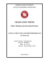
Answers and Solutions: 13 - 7
Sales
Costs
Dollars
Units of Output
(Thousands)
800,000
600,000
400,000
200,000
0 5
10
15 20
Fixed Costs
Sales
Costs
Dollars

Units of Output
(Thousands)
800,000
600,000
400,000
200,000
0 5
10
15 20
Fixed Costs
S
BE
= Q
BE
(P) = (17,500)($31) = $542,500.
The breakeven point increases to 17,500 units because the
contribution margin per each unit sold has decreased.
13-5 a. The current dividend per share, D
0
, = $400,000/200,000 = $2.00. D
1
=
$2.00 (1.05) = $2.10. Therefore, P
0
= D
1
/(k
s
- g) = $2.10/(0.134 - 0.05)
= $25.00.

b. Step 1: Calculate EBIT before the recapitalization:
EBIT = $1,000,000/(1 - T) = $1,000,000/0.6 = $1,666,667.
Note: The firm is 100% equity financed, so there is no
interest expense.
Step 2: Calculate net income after the recapitalization:
[$1,666,667 - 0.11($1,000,000)]0.6 = $934,000.
Step 3: Calculate the number of shares outstanding after the recapi-
talization:
200,000 - ($1,000,000/$25) = 160,000 shares.
Step 4: Calculate D
1
after the recapitalization:
D
0
= 0.4($934,000/160,000) = $2.335.
D
1
= $2.335(1.05) = $2.4518.
Step 5: Calculate P
0
after the recapitalization:
P
0
= D
1
/(k
s
- g) = $2.4518/(0.145 - 0.05) = $25.8079 ≈
$25.81.
13-6 a. LL: D/TA = 30%.

EBIT $4,000,000
Interest ($6,000,000 × 0.10) 600,000
EBT $3,400,000
Tax (40%) 1,360,000
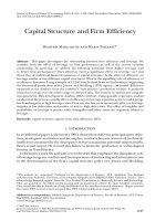
Answers and Solutions: 13 - 8
Sales
Costs
Dollars
Units of Output
(Thousands)
800,000
600,000
400,000
200,000
0 5
10
15 20
Fixed Costs
Net income $2,040,000
Return on equity = $2,040,000/$14,000,000 = 14.6%.
Answers and Solutions: 13 - 9
HL: D/TA = 50%.
EBIT $4,000,000
Interest ($10,000,000 × 0.12) 1,200,000
EBT $2,800,000
Tax (40%) 1,120,000
Net income $1,680,000
Return on equity = $1,680,000/$10,000,000 = 16.8%.
b. LL: D/TA = 60%.
EBIT $4,000,000

Interest ($12,000,000 × 0.15) 1,800,000
EBT $2,200,000
Tax (40%) 880,000
Net income $1,320,000
Return on equity = $1,320,000/$8,000,000 = 16.5%.
Although LL’s return on equity is higher than it was at the 30
percent leverage ratio, it is lower than the 16.8 percent return of
HL.
Initially, as leverage is increased, the return on equity also
increases. But, the interest rate rises when leverage is increased.
Therefore, the return on equity will reach a maximum and then
decline.
13-7 No leverage: D = 0 (debt); E = $14,000,000.
State P
s
EBIT (EBIT - k
d
D)(1-T) ROE
s
P
s
(ROE) P
s
(ROE
s
-RÔE)
2

1 0.2 $4,200,000 $2,520,000 0.18 0.036 0.00113
2 0.5 2,800,000 1,680,000 0.12 0.060 0.00011

3 0.3 700,000 420,000 0.03 0.009 0.00169
RÔE = 0.105
Variance = 0.00293
Standard deviation = 0.054
RÔE = 10.5%.
σ
2
= 0.00293.
σ = 5.4%.
CV = σ/RÔE = 5.4%/10.5% = 0.514.
Leverage ratio = 10%: D = $1,400,000; E = $12,600,000; k
d
= 9%.
State P
s
EBIT (EBIT - k
d
D)(1-T) ROE
s
P
s
(ROE) P
s
(ROE
s
-RÔE)
2

1 0.2 $4,200,000 $2,444,400 0.194 0.039 0.00138
2 0.5 2,800,000 1,604,400 0.127 0.064 0.00013

3 0.3 700,000 344,400 0.027 0.008 0.00212
RÔE = 0.111
Variance = 0.00363
Standard deviation = 0.060
Answers and Solutions: 13 - 10
RÔE = 11.1%.
σ
2
= 0.00363.
σ = 6%.
CV = 6%/11.1% = 0.541.
Leverage ratio = 50%: D = $7,000,000; E = $7,000,000; k
d
= 11%.
State P
s
EBIT (EBIT - k
d
D)(1-T) ROE
s
P
s
(ROE) P
s
(ROE
s
-RÔE)
2

1 0.2 $4,200,000 $2,058,000 0.294 0.059 0.00450

2 0.5 2,800,000 1,218,000 0.174 0.087 0.00045
3 0.3 700,000 (42,000) (0.006) (0.002) 0.00675
RÔE = 0.144
Variance = 0.01170
Standard deviation = 0.108
RÔE = 14.4%.
σ
2
= 0.01170.
σ = 10.8%.
CV = 10.8%/14.4% = 0.750.
Leverage ratio = 60%: D = $8,400,000; E = $5,600,000; k
d
= 14%.
State P
s
EBIT (EBIT - k
d
D)(1-T) ROE
s
P
s
(ROE) P
s
(ROE
s
-RÔE)
2

1 0.2 $4,200,000 $1,814,400 0.324 0.065 0.00699

2 0.5 2,800,000 974,400 0.174 0.087 0.00068
3 0.3 700,000 (285,600) (0.051) (0.015) 0.01060
RÔE = 0.137
Variance = 0.01827
Standard deviation = 0.135
RÔE = 13.7%.
σ
2
= 0.01827.
σ = 13.5%.
CV = 13.5%/13.7% = 0.985 ≈ 0.99.
As leverage increases, the expected return on equity rises up to a
point. But as the risk increases with increased leverage, the cost of
debt rises. So after the return on equity peaks, it then begins to fall.
As leverage increases, the measures of risk (both the standard deviation
and the coefficient of variation of the return on equity) rise with each
increase in leverage.
13-8 Facts as given: Current capital structure: 25%D, 75%E; k
RF
= 5%; k
M
–
k
RF
= 6%; T = 40%; k
s
= 14%.
Step 1: Determine the firm’s current beta.
k
s

= k
RF
+ (k
M
– k
RF
)b
14% = 5% + (6%)b
9% = 6%b
1.5 = b.
Answers and Solutions: 13 - 11
Step 2: Determine the firm’s unlevered beta, b
U
.
b
U
= b
L
/[1 + (1 – T)(D/E)]
b
U
= 1.5/[1 + (1 – 0.4)(0.25/0.75)]
b
U
= 1.5/1.20
b
U
= 1.25.
Answers and Solutions: 13 - 12
Step 3: Determine the firm’s beta under the new capital structure.

b
L
= b
U
(1 + (1 – T)(D/E))
b
L
= 1.25[1 + (1 – 0.4)(0.5/0.5)]
b
L
= 1.25(1.6)
b
L
= 2.
Step 4: Determine the firm’s new cost of equity under the changed
capital structure.
k
s
= k
RF
+ (k
M
– k
RF
)b
k
s
= 5% + (6%)2
k
s

= 17%.
13-9 a. Using the standard formula for the weighted average cost of capital,
we find:
WACC = w
d
k
d
(1 - T) + w
c
k
s
WACC = (0.2)(8%)(1 - 0.4) + (0.8)(12.5%)
WACC = 10.96%.
b. The firm's current levered beta at 20% debt can be found using the
CAPM formula.


k
s
= k
RF
+ (k
M
- k
RF
)b
12.5% = 5% + (6%)b
b = 1.25.
c. To “unlever” the firm's beta, the Hamada Equation is used.

b
L
= b
U
[1 + (1 – T)(D/E)]
1.25 = b
U
[1 + (1 - 0.4)(0.2/0.8)]
1.25 = b
U
(1.15)


b
U
= 1.086957.
d. To determine the firm’s new cost of common equity, one must find the
firm’s new beta under its new capital structure. Consequently, you
must “relever” the firm's beta using the Hamada Equation:
b
L,40%
= b
U
[1 + (1 – T)(D/E)]
b
L,40%
= 1.086957 [1 + (1 - 0.4)(0.4/0.6)]
b
L,40%

= 1.086957(1.4)


b
U
= 1.521739.
The firm's cost of equity, as stated in the problem, is derived using
the CAPM equation.
k
s
= k
RF
+ (k
M
- k
RF
)b
k
s
= 5% + (6%)1.521739
k
s
= 14.13%.
e. Again, the standard formula for the weighted average cost of capital
is used. Remember, the WACC is a marginal, after-tax cost of capital
Answers and Solutions: 13 - 13
and hence the relevant before-tax cost of debt is now 9.5% and the
cost of equity is 14.13%.
WACC = w
d

k
d
(1 - T) + w
c
k
s
WACC = (0.4)(9.5%)(1 - 0.4) + (0.6)(14.13%)
WACC = 10.76%.
f. The firm should be advised to proceed with the recapitalization as
it causes the WACC to decrease from 10.96% to 10.76%. As a result,
the recapitalization would lead to an increase in firm value.
13-10 a. Expected EPS for Firm C:
E(EPS
C
) = 0.1(-$2.40) + 0.2($1.35) + 0.4($5.10) + 0.2($8.85) +
0.1($12.60)
= -$0.24 + $0.27 + $2.04 + $1.77 + $1.26 = $5.10.
(Note that the table values and probabilities are dispersed in a
symmetric manner such that the answer to this problem could have been
obtained by simple inspection.)
b. According to the standard deviations of EPS, Firm B is the least
risky, while C is the riskiest. However, this analysis does not take
account of portfolio effects if C’s earnings go up when most other
companies’ decline (that is, its beta is low), its apparent riskiness
would be reduced. Also, standard deviation is related to size, or
scale, and to correct for scale we could calculate a coefficient of
variation (σ/mean):
E(EPS) σ CV = σ /E(EPS)
A $5.10 $3.61 0.71
B 4.20 2.96 0.70

C 5.10 4.11 0.81
By this criterion, C is still the most risky.
13-11 a. Without new investment
Sales $12,960,000
VC 10,200,000
FC 1,560,000
EBIT $ 1,200,000
Interest 384,000*
EBT $ 816,000
Tax (40%) 326,400
Net income $ 489,600
*Interest = 0.08($4,800,000) = $384,000.
Answers and Solutions: 13 - 14
1. EPS
Old
= $489,600/240,000 = $2.04.
With new investment Debt Stock
Sales $12,960,000 $12,960,000
VC (0.8)($10,200,000) 8,160,000 8,160,000
FC 1,800,000 1,800,000
EBIT $ 3,000,000 $ 3,000,000
Interest 1,104,000** 384,000
EBT $ 1,896,000 $ 2,616,000
Tax (40%) 758,400 1,046,400
Net income $ 1,137,600 $ 1,569,600
**Interest = 0.08($4,800,000) + 0.10($7,200,000) = $1,104,000.
2. EPS
D
= $1,137,600/240,000 = $4.74.
3. EPS

S
= $1,569,600/480,000 = $3.27.
EPS should improve, but expected EPS is significantly higher if
financial leverage is used.
b. EPS =
N
T) - I)(1 - F - VC - (Sales
=
N
T) - I)(1 - F - VQ - (PQ
.
EPS
Debt
=
240,000
)(0.6)$1,104,000 - $1,800,000 - Q$18.133 - Q($28.8
=
240,000
)(0.6)$2,904,000 - Q($10.667
.
EPS
Stock
=
480,000
)(0.6)$2,184,000 - Q($10.667
.
Therefore,
480,000
)(0.6)$2,184,000 - Q($10.667
=

240,000
)(0.6)$2,904,000 - Q(10.667
$10.667Q = $3,624,000
Q = 339,750 units.
This is the “indifference” sales level, where EPS
debt
= EPS
stock
.
c. EPS
Old
=
240,000
0.6)$384,000)( - $1,560,000 - Q$22.667 - Q($28.8
= 0
$6.133Q = $1,944,000
Q = 316,957
units.
This is the Q
BE
considering interest charges.
Answers and Solutions: 13 - 15
EPS
New,Debt
=
240,000
)(0.6)$2,904,000 - Q$18.133 - Q($28.8
= 0
$10.667Q = $2,904,000

Q = 272,250 units.
EPS
New,Stock
=
480,000
)(0.6)$2,184,000 - Q($10.667
= 0
$10.667Q = $2,184,000


Q = 204,750 units.
d. At the expected sales level, 450,000 units, we have these EPS values:
EPS
Old Setup
= $2.04. EPS
New,Debt
= $4.74. EPS
New,Stock
= $3.27.
We are given that operating leverage is lower under the new setup.
Accordingly, this suggests that the new production setup is less
risky than the old one variable costs drop very sharply, while fixed
costs rise less, so the firm has lower costs at “reasonable” sales
levels.
In view of both risk and profit considerations, the new production
setup seems better. Therefore, the question that remains is how to
finance the investment.
The indifference sales level, where EPS
debt

= EPS
stock
, is 339,750
units. This is well below the 450,000 expected sales level. If
sales fall as low as 250,000 units, these EPS figures would result:
EPS
Debt
=
240,000
](0.6)$2,904,000 - ,000)0$18.133(25 - ,000)0[$28.8(25
= -$0.59.
EPS
Stock
=
480,000
](0.6)$2,184,000 - ,000)0$18.133(25 - ,000)0[$28.8(25
= $0.60.
These calculations assume that P and V remain constant, and that the
company can obtain tax credits on losses. Of course, if sales rose
above the expected 450,000 level, EPS would soar if the firm used
debt financing.
In the “real world” we would have more information on which to
base the decision coverage ratios of other companies in the industry
and better estimates of the likely range of unit sales. On the basis
of the information at hand, we would probably use equity financing,
but the decision is really not obvious.
Answers and Solutions: 13 - 16
13-12 Use of debt (millions of dollars):
Probability 0.3 0.4 0.3
Sales $2,250.0 $2,700.0 $3,150.0

EBIT (10%) 225.0 270.0 315.0
Interest* 77.4 77.4 77.4
EBT $ 147.6 $ 192.6 $ 237.6
Taxes (40%) 59.0 77.0 95.0
Net income $ 88.6 $ 115.6 $ 142.6
Earnings per share (20 million shares) $ 4.43 $ 5.78 $ 7.13
*Interest on debt = ($270 × 0.12) + Current interest expense
= $32.4 + $45 = $77.4.
Expected EPS = (0.30)($4.43) + (0.40)($5.78) + (0.30)($7.13)
= $5.78 if debt is used.
σ
2
Debt
= (0.30)($4.43 - $5.78)
2
+ (0.40)($5.78 - $5.78)
2
+ (0.30)($7.13 - $5.78)
2
= 1.094.
σ
Debt
=
094.1
= $1.05
= Standard deviation of EPS if debt financing is used.
CV =
$5.78
$1.05
= 0.18.

E(TIE
Debt
) =
I
E(EBIT)
=
$77.4
$270
= 3.49×.
Debt/Assets = ($652.50 + $300 + $270)/($1,350 + $270) = 75.5%.
Use of stock (millions of dollars):
Probability 0.3 0.4 0.3
Sales $2,250.0 $2,700.0 $3,150.0
EBIT 225.0 270.0 315.0
Interest 45.0 45.0 45.0
EBT $ 180.0 $ 225.0 $ 270.0
Taxes (40%) 72.0 90.0 108.0
Net income $ 108.0 $ 135.0 $ 162.0
Earnings per share
(24.5 million shares)* $ 4.41 $ 5.51 $ 6.61
*Number of shares = ($270 million/$60) + 20 million
= 4.5 million + 20 million = 24.5 million.
EPS
Equity
= (0.30)($4.41) + (0.40)($5.51) + (0.30)($6.61) = $5.51.
σ
2
Equity
= (0.30)($4.41 - $5.51)
2

+ (0.40)($5.51 - $5.51)
2
+ (0.30)($6.61 - $5.51)
2
= 0.7260.
Answers and Solutions: 13 - 17
σ
Equity
=
7260.0
= $0.85.
CV =
$5.51
$0.85
= 0.15.
E(TIE) =
$45
$270
= 6.00×.
Assets
Debt
=
$270 + $1,350
$300 + $652.50
= 58.8%.
Under debt financing the expected EPS is $5.78, the standard deviation
is $1.05, the CV is 0.18, and the debt ratio increases to 75.5 percent.
(The debt ratio had been 70.6 percent.) Under equity financing the
expected EPS is $5.51, the standard deviation is $0.85, the CV is 0.15,
and the debt ratio decreases to 58.8 percent. At this interest rate,

debt financing provides a higher expected EPS than equity financing;
however, the debt ratio is significantly higher under the debt financing
situation as compared with the equity financing situation. Because EPS
is not significantly greater under debt financing, while the risk is
noticeably greater, equity financing should be recommended.
13-13 a. Firm A
1. Fixed costs = $80,000.
2. Variable cost/unit =
units Breakeven
cost Fixed - sales Breakeven
=
./unit$4.80 =
25,000
$120,000
=
25,000
$80,000 - $200,000
3. Selling price/unit =
./unit$8.00 =
25,000
$200,000
=
units Breakeven
sales Breakeven
Firm B
1. Fixed costs = $120,000.
2. Variable cost/unit =
units Breakeven
costs Fixed - sales Breakeven
=

30,000
$120,000 - $240,000
= $4.00/unit.
3. Selling price/unit =
units Breakeven
sales Breakeven
=
30,000
$240,000
= $8.00/unit.
b. Firm B has the higher operating leverage due to its larger amount of
fixed costs.
Answers and Solutions: 13 - 18
c. Operating profit = (Selling price)(Units sold) - Fixed costs
- (Variable costs/unit)(Units sold).
Firm A’s operating profit = $8X - $80,000 - $4.80X.
Firm B’s operating profit = $8X - $120,000 - $4.00X.
Set the two equations equal to each other:
$8X - $80,000 - $4.80X = $8X - $120,000 - $4.00X
-$0.8X = -$40,000
X = $40,000/$0.80 = 50,000 units.
Sales level = (Selling price)(Units) = $8(50,000) = $400,000.
At this sales level, both firms earn $80,000:
Profit
A
= $8(50,000) - $80,000 - $4.80(50,000)


= $400,000 - $80,000 - $240,000 = $80,000.
Profit

B
= $8(50,000) - $120,000 - $4.00(50,000)


= $400,000 - $120,000 - $200,000 = $80,000.
13-14 Tax rate = 40% k
RF
= 5.0%
b
U
= 1.2 k
M
– k
RF
= 6.0%
From data given in the problem and table we can develop the following
table:
Leveraged
D/A E/A D/E k
d
k
d
(1 – T) beta
a
k
s
b
WACC
c
0.00 1.00 0.0000 7.00% 4.20% 1.20 12.20% 12.20%

0.20 0.80 0.2500 8.00 4.80 1.38 13.28 11.58
0.40 0.60 0.6667 10.00 6.00 1.68 15.08 11.45
0.60 0.40 1.5000 12.00 7.20 2.28 18.68 11.79
0.80 0.20 4.0000 15.00 9.00 4.08 29.48 13.10
Notes:
a
These beta estimates were calculated using the Hamada equation, b
L
=
b
U
[1 + (1 – T)(D/E)].
b
These k
s
estimates were calculated using the CAPM, k
s
= k
RF
+ (k
M
–
k
RF
)b.
c
These WACC estimates were calculated with the following equation:
WACC = w
d
(k

d
)(1 – T) + (w
c
)(k
s
).
The firm’s optimal capital structure is that capital structure which
minimizes the firm’s WACC. Elliott’s WACC is minimized at a capital
structure consisting of 40% debt and 60% equity. At that capital
structure, the firm’s WACC is 11.45%.
Answers and Solutions: 13 - 19
13-15 The detailed solution for the spreadsheet problem is available both on
the instructor’s resource CD-ROM and on the instructor’s side of South-
Western’s web site, .
Spreadsheet Problem: 13 - 20
SPREADSHEET PROBLEM
Campus Deli Inc.
Optimal Capital Structure
13-16 ASSUME THAT YOU HAVE JUST BEEN HIRED AS BUSINESS MANAGER OF CAMPUS
DELI (CD), WHICH IS LOCATED ADJACENT TO THE CAMPUS. SALES WERE
$1,100,000 LAST YEAR; VARIABLE COSTS WERE 60 PERCENT OF SALES; AND
FIXED COSTS WERE $40,000. THEREFORE, EBIT TOTALED $400,000. BECAUSE
THE UNIVERSITY’S ENROLLMENT IS CAPPED, EBIT IS EXPECTED TO BE
CONSTANT OVER TIME. SINCE NO EXPANSION CAPITAL IS REQUIRED, CD PAYS
OUT ALL EARNINGS AS DIVIDENDS. ASSETS ARE $2 MILLION, AND 80,000
SHARES ARE OUTSTANDING. THE MANAGEMENT GROUP OWNS ABOUT 50 PERCENT
OF THE STOCK, WHICH IS TRADED IN THE OVER-THE-COUNTER MARKET.
CD CURRENTLY HAS NO DEBT IT IS AN ALL-EQUITY FIRM AND ITS 80,000
SHARES OUTSTANDING SELL AT A PRICE OF $25 PER SHARE, WHICH IS ALSO
THE BOOK VALUE. THE FIRM’S FEDERAL-PLUS-STATE TAX RATE IS 40

PERCENT. ON THE BASIS OF STATEMENTS MADE IN YOUR FINANCE TEXT, YOU
BELIEVE THAT CD’S SHAREHOLDERS WOULD BE BETTER OFF IF SOME DEBT
FINANCING WERE USED. WHEN YOU SUGGESTED THIS TO YOUR NEW BOSS, SHE
ENCOURAGED YOU TO PURSUE THE IDEA, BUT TO PROVIDE SUPPORT FOR THE
SUGGESTION.
IN TODAY’S MARKET, THE RISK-FREE RATE, k
RF
, IS 6 PERCENT AND THE
MARKET RISK PREMIUM, k
M
– k
RF
, IS 6 PERCENT. CD’S UNLEVERED BETA, b
U
,
IS 1.0. SINCE CD CURRENTLY HAS NO DEBT, ITS COST OF EQUITY (AND
WACC) IS 12 PERCENT.
IF THE FIRM WERE RECAPITALIZED, DEBT WOULD BE ISSUED, AND THE
BORROWED FUNDS WOULD BE USED TO REPURCHASE STOCK. STOCKHOLDERS, IN
TURN, WOULD USE FUNDS PROVIDED BY THE REPURCHASE TO BUY EQUITIES IN
OTHER FAST-FOOD COMPANIES SIMILAR TO CD. YOU PLAN TO COMPLETE YOUR
REPORT BY ASKING AND THEN ANSWERING THE FOLLOWING QUESTIONS.
A. 1. WHAT IS BUSINESS RISK? WHAT FACTORS INFLUENCE A FIRM’S BUSINESS
RISK?
Integrated Case: 13 - 21
INTEGRATED CASE
ANSWER: [SHOW S13-1 THROUGH S13-3 HERE.] BUSINESS RISK IS THE RISKINESS
INHERENT IN THE FIRM’S OPERATIONS IF IT USES NO DEBT. A FIRM’S
BUSINESS RISK IS AFFECTED BY MANY FACTORS, INCLUDING THESE:
(1) VARIABILITY IN THE DEMAND FOR ITS OUTPUT, (2) VARIABILITY IN THE

PRICE AT WHICH ITS OUTPUT CAN BE SOLD, (3) VARIABILITY IN THE PRICES
OF ITS INPUTS, (4) THE FIRM’S ABILITY TO ADJUST OUTPUT PRICES AS
INPUT PRICES CHANGE, (5) THE AMOUNT OF OPERATING LEVERAGE USED BY THE
FIRM, AND (6) SPECIAL RISK FACTORS (SUCH AS POTENTIAL PRODUCT
LIABILITY FOR A DRUG COMPANY OR THE POTENTIAL COST OF A NUCLEAR
ACCIDENT FOR A UTILITY WITH NUCLEAR PLANTS).
A. 2. WHAT IS OPERATING LEVERAGE, AND HOW DOES IT AFFECT A FIRM’S BUSINESS
RISK?
ANSWER: [SHOW S13-4 THROUGH S13-6 HERE.] OPERATING LEVERAGE IS THE EXTENT TO
WHICH FIXED COSTS ARE USED IN A FIRM’S OPERATIONS. IF A HIGH
PERCENTAGE OF THE FIRM’S TOTAL COSTS ARE FIXED, AND HENCE DO NOT
DECLINE WHEN DEMAND FALLS, THEN THE FIRM IS SAID TO HAVE HIGH
OPERATING LEVERAGE. OTHER THINGS HELD CONSTANT, THE GREATER A FIRM’S
OPERATING LEVERAGE, THE GREATER ITS BUSINESS RISK.
B. 1. WHAT IS MEANT BY THE TERMS “FINANCIAL LEVERAGE” AND “FINANCIAL RISK”?
ANSWER: [SHOW S13-7 HERE.] FINANCIAL LEVERAGE REFERS TO THE FIRM’S DECISION
TO FINANCE WITH FIXED-CHARGE SECURITIES, SUCH AS DEBT AND PREFERRED
STOCK. FINANCIAL RISK IS THE ADDITIONAL RISK, OVER AND ABOVE THE
COMPANY’S INHERENT BUSINESS RISK, BORNE BY THE STOCKHOLDERS AS A
RESULT OF THE FIRM’S DECISION TO FINANCE WITH DEBT.
B. 2. HOW DOES FINANCIAL RISK DIFFER FROM BUSINESS RISK?
ANSWER: [SHOW S13-8 HERE.] AS WE DISCUSSED ABOVE, BUSINESS RISK DEPENDS ON A
NUMBER OF FACTORS SUCH AS SALES AND COST VARIABILITY, AND OPERATING
LEVERAGE. FINANCIAL RISK, ON THE OTHER HAND, DEPENDS ON ONLY ONE
FACTOR THE AMOUNT OF FIXED-CHARGE CAPITAL THE COMPANY USES.
Integrated Case: 13 - 22
C. NOW, TO DEVELOP AN EXAMPLE THAT CAN BE PRESENTED TO CD’S MANAGEMENT
AS AN ILLUSTRATION, CONSIDER TWO HYPOTHETICAL FIRMS, FIRM U, WITH
ZERO DEBT FINANCING, AND FIRM L, WITH $10,000 OF 12 PERCENT DEBT.
BOTH FIRMS HAVE $20,000 IN TOTAL ASSETS AND A 40 PERCENT FEDERAL-

PLUS-STATE TAX RATE, AND THEY HAVE THE FOLLOWING EBIT PROBABILITY
DISTRIBUTION FOR NEXT YEAR:
PROBABILITY EBIT
0.25 $2,000
0.50 3,000
0.25 4,000
1. COMPLETE THE PARTIAL INCOME STATEMENTS AND THE FIRMS’ RATIOS IN TABLE
IC13-1.
TABLE IC13-1. INCOME STATEMENTS AND RATIOS
FIRM U FIRM L
ASSETS $20,000 $20,000 $20,000 $20,000 $20,000 $20,000
EQUITY $20,000 $20,000 $20,000 $10,000 $10,000 $10,000
PROBABILITY 0.25 0.50 0.25 0.25 0.50 0.25
SALES $ 6,000 $ 9,000 $12,000 $ 6,000 $ 9,000 $12,000
OPER. COSTS 4,000 6,000 8,000 4,000 6,000 8,000
EBIT $ 2,000 $ 3,000 $ 4,000 $ 2,000 $ 3,000 $ 4,000
INT. (12%) 0 0 0 1,200 1,200
EBT $ 2,000 $ 3,000 $ 4,000 $ 800 $ $ 2,800
TAXES (40%) 800 1,200 1,600 320 1,120
NET INCOME $ 1,200 $ 1,800 $ 2,400 $ 480 $ $ 1,680
BEP 10.0% 15.0% 20.0% 10.0% % 20.0%
ROE 6.0% 9.0% 12.0% 4.8% % 16.8%
TIE ∞ ∞ ∞ 1.7× × 3.3×
E(BEP) 15.0% %
E(ROE) 9.0% 10.8%
E(TIE) ∞ 2.5×
SD(BEP) 3.5% %
SD(ROE) 2.1% 4.2%
SD(TIE) 0 0.6×
Integrated Case: 13 - 23

ANSWER: [SHOW S13-9 THROUGH S13-12 HERE.] HERE ARE THE FULLY COMPLETED
STATEMENTS:
FIRM U FIRM L
ASSETS $20,000 $20,000 $20,000 $20,000 $20,000 $20,000
EQUITY $20,000 $20,000 $20,000 $10,000 $10,000 $10,000
EBIT $ 2,000 $ 3,000 $ 4,000 $ 2,000 $ 3,000 $ 4,000
I (12%) 0 0 0 1,200 1,200 1,200
EBT $ 2,000 $ 3,000 $ 4,000 $ 800 $ 1,800 $ 2,800
TAXES (40%) 800 1,200 1,600 320 720 1,120
NI $ 1,200 $ 1,800 $ 2,400 $ 480 $ 1,080 $ 1,680
BEP 10.0% 15.0% 20.0% 10.0% 15.0% 20.0%
ROE 6.0% 9.0% 12.0% 4.8% 10.8% 16.8%
TIE ∞ ∞

∞ 1.7× 2.5× 3.3×
E(BEP) 15.0% 15.0%
E(ROE) 9.0% 10.8%
E(TIE) ∞ 2.5×
SD(BEP) 3.5% 3.5%
SD(ROE) 2.1% 4.2%
SD(TIE) 0 0.6×
C. 2. BE PREPARED TO DISCUSS EACH ENTRY IN THE TABLE AND TO EXPLAIN HOW
THIS EXAMPLE ILLUSTRATES THE IMPACT OF FINANCIAL LEVERAGE ON EXPECTED
RATE OF RETURN AND RISK.
ANSWER: [SHOW S13-13 THROUGH S13-15 HERE.] CONCLUSIONS FROM THE ANALYSIS:
1. THE FIRM’S BASIC EARNING POWER, BEP = EBIT/TOTAL ASSETS, IS
UNAFFECTED BY FINANCIAL LEVERAGE.
2. FIRM L HAS THE HIGHER EXPECTED ROE:
E(ROE
U

) = 0.25(6.0%) + 0.50(9.0%) + 0.25(12.0%) = 9.0%.
E(ROE
L
) = 0.25(4.8%) + 0.50(10.8%) + 0.25(16.8%) = 10.8%.
THEREFORE, THE USE OF FINANCIAL LEVERAGE HAS INCREASED THE
EXPECTED PROFITABILITY TO SHAREHOLDERS. TAX SAVINGS CAUSE THE
HIGHER EXPECTED ROE
L
. (IF THE FIRM USES DEBT, THE STOCK IS
RISKIER, WHICH THEN CAUSES k
d
AND k
s
TO INCREASE. WITH A HIGHER
k
d
, INTEREST INCREASES, SO THE INTEREST TAX SAVINGS INCREASES.)
Integrated Case: 13 - 24
3. FIRM L HAS A WIDER RANGE OF ROEs, AND A HIGHER STANDARD DEVIATION
OF ROE, INDICATING THAT ITS HIGHER EXPECTED RETURN IS ACCOMPANIED
BY HIGHER RISK. TO BE PRECISE:
σ
ROE (UNLEVERED)
= 2.12%, AND CV = 0.24.
σ
ROE (LEVERED)
= 4.24%, AND CV = 0.39.
THUS, IN A STAND-ALONE RISK SENSE, FIRM L IS TWICE AS RISKY AS
FIRM U ITS BUSINESS RISK IS 2.12 PERCENT, BUT ITS STAND-ALONE
RISK IS 4.24 PERCENT, SO ITS FINANCIAL RISK IS 4.24% - 2.12% =

2.12%.
4. WHEN EBIT = $2,000, ROE
U
> ROE
L
, AND LEVERAGE HAS A NEGATIVE
IMPACT ON PROFITABILITY. HOWEVER, AT THE EXPECTED LEVEL OF EBIT,
ROE
L
> ROE
U
.
5. LEVERAGE WILL ALWAYS BOOST EXPECTED ROE IF THE EXPECTED UNLEVERED
ROA EXCEEDS THE AFTER-TAX COST OF DEBT. HERE E(ROA) = E(UNLEVERED
ROE) = 9.0% > k
d
(1 - T) = 12%(0.6) = 7.2%, SO THE USE OF DEBT
RAISES EXPECTED ROE.
6. FINALLY, NOTE THAT THE TIE RATIO IS HUGE (UNDEFINED, OR INFINITELY
LARGE) IF NO DEBT IS USED, BUT IT IS RELATIVELY LOW IF 50 PERCENT
DEBT IS USED. THE EXPECTED TIE WOULD BE LARGER THAN 2.5× IF LESS
DEBT WERE USED, BUT SMALLER IF LEVERAGE WERE INCREASED.
D. AFTER SPEAKING WITH A LOCAL INVESTMENT BANKER, YOU OBTAIN THE
FOLLOWING ESTIMATES OF THE COST OF DEBT AT DIFFERENT DEBT LEVELS (IN
THOUSANDS OF DOLLARS):
AMOUNT DEBT/ASSETS DEBT/EQUITY BOND
BORROWED RATIO RATIO RATING k
d
$ 0 0.000 0.0000
250 0.125 0.1429 AA 8.0%

500 0.250 0.3333 A 9.0
750 0.375 0.6000 BBB 11.5
1,000 0.500 1.0000 BB 14.0
NOW CONSIDER THE OPTIMAL CAPITAL STRUCTURE FOR CD.
Integrated Case: 13 - 25