Real Options in practice Chapter 2 pot
Bạn đang xem bản rút gọn của tài liệu. Xem và tải ngay bản đầy đủ của tài liệu tại đây (340.33 KB, 34 trang )
33
CHAPTER
2
Taking an Idea
into Practice
REAL OPTION CONCEPTS AND APPLICATIONS
Real option analysis values and rewards managerial insight and the result-
ing flexibility. Managers may delay an investment until further information
is available to provide better insights into market conditions. They may
change the scale of an ongoing project by either downsizing or expanding it.
They may decide to abandon a project altogether. They may decide to ex-
change input resources, that is, switch from one energy form to another, or
from one product output to another. They may also decide to structure an
investment into a major new project in incremental steps, with an option to
grow at each step, while at the same time obtaining valuable market and
product information. Finally, they may want to stage a very risky investment
into a new technology or into a new prototype incorporating multiple “go”
and “no-go” decision points based on conditional probabilities of achieving
certain milestones along the way.
The initial real option work focused on the value created by abandon-
ing a project and liquidating the assets.
1
A project that can be abandoned, so
the reasoning goes, is in essence an American put option on a dividend-
paying stock: It gives management the right but entails no obligation to sell
the asset at a salvage price, the exercise price, at any time, but it will forego
the cash flows generated by the asset, equivalent to the dividend on a stock,
as shown in Figure 2.1.
This managerial flexibility has value, and the value can be determined
using option pricing theory. Management will make use of the abandonment
option once market conditions have deteriorated and the potential value cre-
ated by the asset, such as a production plant or an airplane fleet, over its re-
maining lifetime is lower than the value created by selling it. The value of the
put is the salvage price minus the costs incurred to exercise the option, such
as transaction costs minus revenues foregone by selling the asset.
The first call on real assets to be priced was an investment in a natural
resource project such as the exploration of an oil field or a mine.
2
Owning
the mine provides the owner with a call option, the right, but not the oblig-
ation, to explore the mine. The value of the call on the mine depends on the
costs and resources required to recover its contents but also on the revenue
stream to be generated by future sales. The decision as to whether to initi-
ate or continue exploration, to slow down exploration, or to shut down the
mine altogether will be guided by management’s expectations of future mar-
ket conditions, as shown in Figure 2.2. The value of the option on the mine
today reflects the degree of managerial flexibility in place to respond to fu-
ture uncertainties in the optimum fashion.
This work also created the important insight that there is value in wait-
ing. Traditional NPV analysis recommends investing as soon as today’s
value of expected future payoffs is bigger than today’s value of the expected
costs. In contrast, option analysis argues that there is value in waiting and
deferring the investment decision until further information arrives to solve
external market uncertainties, as shown in Figure 2.3.
Investing today in an uncertain future, where markets can be either
great or bad, implies that resources are irreversibly spent while the payoff is
uncertain. Deferring the investment until market uncertainty has been re-
34 REAL OPTIONS IN PRACTICE
Shut-Down
1
2
3
Prices
Costs
Profit
Salvage Value
FIGURE 2.1 The abandonment option
solved and then reserving the right, or the option, to invest only when mar-
ket conditions are excellent, implies that the upside potential of the market
can be taken advantage of while the downside risk resulting from bad mar-
ket conditions is eliminated. Herein lies the value of waiting.
3
MacDonald
and Siegel MacDonald
4
were the first to recognize the connection between
irreversibility and uncertainty. They made the point that committing re-
sources irreversibly into an uncertain future requires an option premium that
compensates for the loss of flexibility in the face of uncertainty.
Majd and Pindyck
5
were the first to propose an option pricing model
that includes the value created by managerial flexibility during the course of
Taking an Idea into Practice 35
3
1
2
Future Market
Condition
Growing Demand
Low Demand
Too Much Supply
Substitution by
Other Product
Managerial
Flexibility
Expand
Slow Down/
Mothball
Shut Down
Value
Proposition
Option Cone
0
Today’s
Value
FIGURE 2.2 The real option cone for a mine owner
2
1
Great Market
Bad Market
Invest
Now
Invest Only
When Market Is Great
Option Cone
0
Wait
Observe
Face Market
Expected
Payoff
Bad Market Great Market
Bad Market Great Market
FIGURE 2.3 The value of waiting to invest
a prolonged staged investment project: Depending on new information ar-
riving from the market, management can accelerate or slow down the pro-
ject and also abandon it. Further, they pointed out that in such a sequential
project each dollar spent buys the option to spend the next dollar, while cash
flows only happen after the project is completed. This lays the conceptual
groundwork for the compound option, which we will describe in more de-
tail below. The important insights derived from the Majd and Pindyck study
are the following: (i) Within a sequential project, the value of the investment
program changes as a function of the value of the completed project, which
is likely to fluctuate over a long “time-to-build” time period as well as the
outstanding investment cost K required to complete the project. For each se-
quential phase the authors derive the critical project value of the completed
project that needs to be met to justify going forward with resource invest-
ment into the next phase. (ii) This critical investment value of the completed
project depends on the opportunity cost of money and increases with the as-
sumed volatility of the completed project.
The work by Majd and Pindyck confirmed and extended the basic con-
cept brought about by others earlier,
6
namely, that growing uncertainty in-
creases the value of the call option and thereby the incentive to hold the
option while decreasing the incentive to exercise it by investing. The most
important insight of the Majd and Pindyck study is that time to build re-
duces the value of the payoff at completion, and that loss increases as the op-
portunity cost of delaying increases, further increasing the critical value to
invest. Opportunity cost is, for example, foregone revenue: the longer it
takes to complete the project, the more the potential revenue stream is fore-
gone. For such a scenario, two main drivers of the option value emerge: the
volatility or uncertainty of future cash flows, which increases the critical
threshold to invest, and the rate of opportunity cost, which decreases it, as
shown in Figure 2.4.
However, the effect of the opportunity costs also depends on the volatil-
ity. Time to build reduces the expected payoff at completion and creates op-
portunity costs, that is, revenue foregone due to the time it takes to complete
the project. With low project volatility and high opportunity costs the in-
centive to invest declines. As project volatility increases, opportunity costs
further increase and tend to lower the critical threshold to invest.
Depending on prevailing market conditions, managers routinely adjust
the scale of an existing operation. For example, in a manufacturing plant
there is flexibility to expand or to contract production to adjust to demand.
Likewise, management can adjust the output of a mine or an oilfield to ad-
just to seasonal or macroeconomic changes in the market place. Brennan
and Schwartz were the first to value the flexibility of being able to respond
to those changes, and others extended that concept.
7
Expansion and con-
36 REAL OPTIONS IN PRACTICE
tracting options relate not just to manufacturing or natural resource invest-
ments. Any joint venture that turns into an acquisition strategy qualifies as
an expansion strategy. As empirical data based on the analysis of ninety-two
joint ventures suggest, exercise of the option to expand from a joint venture
into an acquisition is triggered by a perceived increase of the venture market
value in response to product-market signals.
8
If management receives signals
from the market to suggest significant growth in product demand and there-
fore an increase in the value of the venture, it becomes more inclined to ex-
pand the joint venture option into an acquisition.
Managers also have the flexibility to exchange one product for another,
to alter input parameters, or to change the speed of production. This flexi-
bility has been named the “exchange option.” For example, oil refineries
may produce crude heating oil or gasoline,
9
and the production output mix
will be guided by what is perceived to be the most profitable mix. A plant that
is allowed to implement production flexibility creates switching value. While
management will not know which product will be most profitable in the fu-
ture, a flexible plant creates the infrastructure to preserve future flexibility,
thereby allowing management to respond to future uncertainties in the opti-
mal fashion.
10
This is very similar to the real option we described earlier, in-
volving heating oil and natural gas, encountered by the home owner.
The decision to enter new emerging markets involves considerable risk
and uncertainty, and is likely to give a negative NPV in a traditional dis-
counted cash flow analysis. However, this initial investment also lays the foun-
dation for future market expansion, should the initial entry be successful.
Taking an Idea into Practice 37
Invest
Now
Collect
RevenueFace Market
Option
Cones
0
Wait
Observe
Expected
Payoff
Revenue
Volatility
Critical Value to Invest
Volatility
Critical Value to Invest
Opportunity Cost
FIGURE 2.4 The critical cost while waiting to invest
Hence, the initial investment buys the corporation the option to grow, and the
future market potential created by establishing an initial foreign subsidiary
needs to be included in the original project appraisal. Several authors engaged
in pioneering work related to value growth options between 1977 and 1988.
11
Practical examples include the investment in information technology infra-
structure, R&D projects, or expansion into other markets that can be staged
in segmental steps.
12
Anheuser Busch
13
notably created $13.4 billion in value
in two years by expanding its investments by $1.9 billion. More than half of
the value creation, namely 51%, is attributed to growth options that Anheuser
acquired by obtaining minority interests in existing brewing concerns located
in parts of the world with high growth rates for beer demand. Under the terms
of the agreement, the local concern distributes Anheuser Busch products in
these markets, effectively creating growth options for Anheuser Busch. The
joint ventures allow Anheuser Busch to test and understand the local markets
before committing larger investments toa more aggressive expansion strategy
in those regions that prove most profitable.
The concept of compounded options is immediately attractive to an
R&D project that comes in several phases, with each phase relying on suc-
cessful completion of the previous phase. The investment will only be com-
pleted once all phases have been completed successfully, and only then can
cash flows be realized. However, each completed phase contributes to the
continuous value appreciation through two components: by reducing over-
all project uncertainty that is highest at the beginning,
14
but also by creating
information, knowledge, expertise, and insight that may be transferable to
other related projects, even if this one fails. Not surprisingly, therefore, com-
pounded real options were quickly adapted in high-tech high-risk industries
with a rich portfolio of R&D projects but also were adapted to applications
in strategy and operations.
15
EXTENSION AND VARIATIONS OF
THE CONCEPTS—NEW INSIGHTS
As applications of real options spread, the basic concepts are fine-tuned.
Novel option concepts continue to emerge, and existing paradigms are
changed and extended. Initial option work studied mostly the impact of
market uncertainty on option valuation and the timing and extent of invest-
ment decisions. The critical value to invest was defined by the cost of in-
vestment, the future asset value and the option premium, or the value of
waiting to invest to reduce future uncertainty.
16
Trigeorgis
17
was the first to
38 REAL OPTIONS IN PRACTICE
point out that a single investment project often entails several distinct real
options creating scope for multiple option interactions. Once multiple op-
tions come into play, the value of each individual option tends to increase;
but taken together, depending on the individual scenario, those embedded
options may add up, synergize, or antagonize in terms of their contribution
to the overall option value of the investment project.
While the concept of waiting and the value of sequential investment in
the face of uncertainty has gained much attention, the notion that new in-
formation obtained through learning may also impact on the value of an
investment is less explored.
18
This work opens a different perspective on op-
tion valuation. Option value derives from obtaining better information by
delaying a decision, whereas, on the contrary, making the decision today
could result in irreversible loss, an idea pioneered in the early seventies.
19
Arrow and Fisher then looked into the valuation of an irreversible invest-
ment decision, namely, the development of a piece of land that will forever
change the natural features of an area. The value of the option derives from
information that reduces the variability of the future payoff, creating the
“quasi-option.” In this framework, the option is on the expected value of re-
duced damage, relative to doing nothing. The option value reflects the value
of delaying an irreversible investment that might be harmful and cause irre-
versible damage if additional information is expected in the future that re-
solves current uncertainty and has the potential to alter the course of this
decision—thereby preventing that damage.
The intricate relationship between irreversibility and uncertainty has
featured prominently in environmental economics since the early seventies.
At that time two landmark publications appeared,
20
both of which empha-
sized the irreversibility effect of investment decisions. The standard example
of the “irreversibility effect” is the construction of a dam that irreversibly
floods and destroys a natural valley. In a more general context, this work, as
well as more recent work building on the earlier insights,
21
extends the con-
cept to scenarios in which irreversible decisions are made today even though
preferences may change in the future. That change of preference may result
from new, unanticipated information.
For example, the hazardous effects of lead on human health changed con-
sumer preference for paints. The decision to incorporate lead into paints was
made unknowingly and without anticipating that in the future the world
would be aware of the fact that lead imposes a serious health hazard. A de-
cision maker does not know how many possible future situations she may
overlook, inadvertently. This situation is referred to as hard uncertainty.
Consider the binomial asset tree in Figure 2.5. The decision on the
components of paint is made today, at node 1. In the future, lead may be
Taking an Idea into Practice 39
nonhazardous (node 2), or hazardous (node 3). Suppose that the decision
would be deferred to the later time point t
2
. At t
2
it is known whether lead
is hazardous or not. The quasi-option then values the information gain that
leads to the decision at t
2
, on the condition that no decision was made in t
1
.
In other words, waiting and deferring the decision to t
2
preserves the flexi-
bility to wait for more information before choosing the paint component at
t
2
, and the option value is the value of this flexibility. In such a scenario the
quasi-option is the gain from acquiring or obtaining information relevant to
the state of the world in the decision-making process. If the lead turns out to
be non-hazardous (node 2), the information gain for the decision is imma-
terial; the expected value of the information is the same irrespective of
whether the decision was made at t
1
or t
2
(node 4). On the contrary, if lead
turns out to be hazardous (node 3), the value of that information is mater-
ial; it allows the decision maker who has deferred the decision until the ar-
rival of information at time t
2
to make an informed decision (node 6), while
the decision maker who has committed at t
1
now faces the consequences of
his irreversible decision made in the face of uncertainty and the absence of
information at t
1
(node 7).
In a corporate context, the time value of waiting is meaningful for mo-
nopoly options but needs to be revisited for shared options in a competitive
environment. The value of waiting ignores and potentially compromises the
40 REAL OPTIONS IN PRACTICE
1
3
2
Non-Hazardous
Hazardous
Arrival of
Information
t
1
t
2
Decision
D
2
D
ecision
D
1
V
E
of Future
Information D
1
5
7
6
4
V
E
of Future
Information D
2
V
E
of Future
Information D
1
= D
2
FIGURE 2.5 The quasi-option: facing hard uncertainty
value created by competitive positioning or preemptive moves that might in
fact destroy the value of waiting. In 1994, Dixit and Pindyck took a first
look at a duopoly situation with much simplified assumptions: The scenario
is one in which there is a perpetual option, and both players have the same
set of complete information. Lambrecht and Perraudin
22
extended the con-
cept by introducing American put options as the payoff. They also assumed
that the exercise price of the put was the transaction costs and known only
by the players. The same authors provided an additional extension in a sub-
sequent study.
23
Here, the value of the option to preempt a competitor was
introduced. Again, the option was perpetual in nature, but the authors con-
sidered that each player had no knowledge of the critical value to invest of
the other player. Further, the authors assumed that whoever was second lost
the investment opportunity. Such a scenario is likely to play out only in in-
dustries with strong intellectual property positions. Adding another flavor to
the competitive scenario, the market share lost by deferring an investment
decision can be interpreted as a “competitive dividend,” an opportunity cost
foregone due to later market entry.
24
Not waiting, but investing early and
thereby creating a preemptive position, on the other hand, adds to the divi-
dend yield and hence reduces the critical value to invest. This additional div-
idend, the “competitive dividend,” can be likened to the cash dividend that
is reserved only for the stockholder but is lost by the option holder on the
same stock.
Equally important is the distinction between market uncertainty and
technical or private uncertainty, which relates to the internal capabilities and
skill sets within any given firm to actually carry out successfully an innova-
tion and implement it. Waiting to invest may resolve market uncertainty; it
may even help to observe competitors solving some basic technical uncer-
tainty. But the private, firm-specific source of technical uncertainty cannot
be resolved without investing. Only by committing resources and actually
initiating the project will the firm find out whether it has the skills to ac-
complish the goal.
Initial real option models also assumed that costs were deterministic,
while, in practice, costs are uncertain most of the time, too. For example,
consider a car manufacturer about to embark on building a new plant to
manufacture cars. It will take about two years to complete the project, and
during this time the costs for labor and materials may fluctuate considerably.
Additional uncertainty may stem from changes in government regulations
that may impose further construction and safety or environmental protec-
tion features that imply additional costs. The exact time frame needed to
complete the work is also uncertain. The firm therefore faces significant cost
uncertainties in undertaking the project. In 1993, Pindyck introduced cost
uncertainty as a distinguishing feature of the real option framework.
25
He
Taking an Idea into Practice 41
stated that each dollar spent towards completion really represents a single
investment opportunity with an uncertain outcome, and that each dollar
spent towards completion creates value in the form of the amount of
progress that results. Further, once the new car production plant is com-
pleted, the asset is put in place and generates cash flows, but both demand
and prices will change. During the lifetime of the plant, the demand for cars
will fluctuate, as will the prices for the cars. Further, the firm will move
along a firm-specific learning curve that permits unit cost to fall with expe-
rience and with output. Real option pricing models need to incorporate sto-
chastic product life cycles and changing cost structures that are not
necessarily log-normally distributed. Bollen provided the real option litera-
ture with such a life-cycle model of product demand and unit costs.
26
Time to maturity is a key parameter that drives value in financial op-
tions. Rarely do real options resemble European options with fixed exercise
dates. More often, the exercise time is unknown and very uncertain. For ex-
ample, the time it takes to complete a major project, such as the construction
of a high-rise tower, the design of a new airplane prototype, or a drug de-
velopment project, is uncertain. A competitive entry may unexpectedly kill
all or most of the option value, and the timing of such an entry is also un-
certain. Uncertain time to maturity affects both the time and level of prof-
itability.
27
Uncertainty surrounding the time needed to implement a project
may provoke management to invest very early, especially if resolution of the
timing uncertainty has a strong impact on the profitability of the project.
Specific cases have been investigated in which the first to implement would
be rewarded with a patent and hence could enjoy a monopoly situation for
a limited period of time.
Future asset values are driven not just by product features and market
demand, but also by distribution channels and marketing capabilities. These
important yet uncertain parameters of future asset value were not included
in the early option work. Another fundamental assumption of real option
pricing of investment decisions is that these investments are irreversible,
sunk cost.
28
However, in reality, an investment may not be entirely irre-
versible but may in fact be partially reversible.
29
Within any given firm that
has multiple real options but limited resources, real option analysis has been
used to prioritize among mutually exclusive R&D projects
30
as well as to as-
sist in product portfolio management.
31
Further, the notion that real assets do not move like Brownian motions
but are subject to “catastrophic” events infiltrated much of the option work.
It prompted the development of alternative models to incorporate those ran-
dom events that—after all—are significant drivers of the asset value. Those
random events could be internal discoveries, such as in an R&D project, or
exogenous “catastrophic” events, such as the issue of a competitor’s block-
42 REAL OPTIONS IN PRACTICE
ing patent. Those random events can be modeled as a Poisson process and
linked to market data.
32
Others have enriched the option literature with
Poisson or jump models that represent technology innovations, R&D inno-
vations, or cost-reducing innovations.
33
The application of real option valuation has been extended to value in-
vestments in intangible real assets such as the acquisition of knowledge and
information, and intellectual property, which are sometimes referred to
collectively as virtual options. Another line of research touches on organi-
zational aspects of real option implementation, such as the ability of the
organization to execute real options, specifically the abandonment option,
as well as on the use of real option concepts to create and guide behavior.
COMPARATIVE ANALYSIS:
FINANCIAL AND REAL OPTIONS
The conceptual analogy between financial options and real options is quite
intuitive, and the table in Figure 2.6 summarizes the analogies that can be
easily drawn.
It appears less obvious, however, that the mathematical concepts used to
price financial options—with all the assumptions they rely on—will also be
applicable to real options. The past decade has seen an explosion in real op-
tion developments far beyond the initial basic option concepts (wait/defer,
abandon, switch, grow, expand/contract, compound). This work has delivered
further important insights into the commonalities and differences between
real options and financial options.
Taking an Idea into Practice 43
FIGURE 2.6 Financial versus real options
ANALOGIES: FINANCIAL OPTIONS—REAL OPTIONS
Financial Option Variable Investment Project/Real Option
Exercise price K Costs to acquire the asset
Stock price S Present value of future cash flows
from the asset
Time to expiration t Length of time option is viable
Variance of stock returns s
2
Riskiness of the asset, variance of
the best and worst case scenario
Risk-free rate of return r Risk-free rate of return
Financial options are available on a large and diverse group of underly-
ing assets including individual stocks, stock indexes, government bonds,
currencies, precious metals, and futures contracts. Real options deal with
capital budgeting, investment decisions, and business transactions. The com-
monalities between the two include the following generic basics:
1. Investment in uncertainty
2. Irreversibility
3. The ability to choose between two or more alternatives
Investment decisions in both the financial and in the real world boil
down to answering three key questions: Whether? When? How much? The
dissimilarities between the two, however, outnumber the similarities by far,
and they are quite fundamental. First, there are conceptual dissimilarities.
Decisions must be made on real options even if not all of the uncertainty has
been resolved. In contrast, for financial options, by the time the exercise date
approaches, all variables required to make an informed decision are known.
During the lifetime of an option, it easily moves in, out, and at the money.
The financial option holder observes passively those movements. The real
option holder, in contrast, has the flexibility and the capability—as well as
the obligation towards her shareholders—to impact the movements of the
underlying asset and thereby mitigate the downside risk while preserving or
expanding the upside potential. This falls within the realm of real option ex-
ecution. Hedging of real options is truly a challenge. This imposes restric-
tions as to how much of the downside risk can be truly limited, asking for
prudent assumptions when framing the option analysis. Financial options
have a known time to maturity, while real options most often do not. Mostly,
there is no deadline for a decision to be made, and the time frame during
which the opportunity is alive is often not known. For example, we cannot
say for sure how long it may take to develop a prototype and we do not know
when competitive entry will terminate our option externally and prematurely.
The source of option value is also different for financial and for real op-
tions. For financial options the value of the option is easily determined as the
numerical difference between the upside potential and exercise price. For
real options, part of the value arises naturally for a given firm as a result of
core competence, existing market or technology position, possible barriers
of entry including existing intellectual property, acquired knowledge and ex-
perience, technical expertise, or an existing brand name. Often, part of the
value must be purchased by investments into R&D, intellectual property,
technology development programs, infrastructure, contractual agreements
with others including deals, leases, licensing agreements or outsourcing
agreements.
44 REAL OPTIONS IN PRACTICE
The value of financial and real options responds differently to changes in
certain parameters. For example, the time to maturation increases the value
of the financial option. The intuition behind this is that, with larger time hori-
zons, uncertainty and hence the upside potential increase. For real options, it
depends on whether the option is proprietary or shared. Only in the former
case may the option value increase with time. In the latter scenario, under
competitive threats and at risk of losing market share by late entry, giving up
preemptive and positioning value, and seeing a patent expire, the relationship
between time to maturity and real option value is much more complex.
Financial option value increases with volatility, as higher volatility im-
plies higher upside potential. This does not necessarily apply to real options;
market volatility may increase the value of the option. However, if the main
contribution to the option value comes from strategic preemption, demand
uncertainty will actually pull the plug on the value of the option.
34
Increas-
ing technical volatility, too, may well diminish the option value.
35
Financial options can be leveraged, real options not so easily. Financial
options are traded in centralized markets with complete information for all
players, they are liquid, and their movements are continuous and can be ob-
served at all times. The value of a real asset is hard to monitor continuously;
past movements of the asset are not necessarily indicative of future value dis-
tributions. Real assets are liquid only very limited, and rarely traded. If so,
the markets are decentralized, and information is asymmetric. This makes it
conceptually harder to adapt the no-arbitrage argument to the real option
world—but we ought not to forget that the DCF approach faces the same
challenges.
In the real world, the value of the option can be defined as the difference
between the maximum return from a flexible investment program versus the
return from an inflexible program.
36
Such an analysis reveals the value of
embedded options. For financial options, the strike price is fixed, while for
real options it is often unclear at what cost the option acquisition will come.
The value of the real option will also depend on how uncertain costs and un-
certain future cash flows correlate. We will analyze this in more detail later.
Financial and real options also have distinct exercise rules. These rules
are well defined for financial options. They reflect the underlying mathemat-
ics, which are equally well defined. For example, never exercise an American
option on a non-dividend paying stock. As for real options, the exercise rules
are equally well defined, but the branches of the binomial tree are multiple
and intricately interwoven, making it more complex in defining how uncer-
tainties and flexibility will influence the expected payoff. For real options the
world is a lot fuzzier than for financial options, in which the asset value is
clearly observable at the time of exercise, and time to expiration and exer-
cise price are well defined. For real options, the time horizon tends to be
Taking an Idea into Practice 45
much longer, and both exercise price and asset value are evolving over the
time to maturity, which is uncertain. Realizing the value of a real option
hinges on the ability to execute the option rationally. Financial options tend
to be exercised by rational investors. As to the exercise of real options, or-
ganizational incentive structures, agency conflicts, and “emotional attach-
ments” may stand in the way of rational exercise.
How then can the concepts of financial option pricing still be applied to
real option pricing? Fundamentally, the price of an option reflects the ex-
pected future payoff of the underlying asset at the time of exercise. The
expected future payoff is discounted back to today’s time at the risk-free rate
and gives today’s option value. The procedure rests on the assumption that
in complete markets the investor will find a traded security that exactly
mimics the risk and uncertainties of the option payoff at any point in time
between acquisition and exercise of the option. Using the twin security and
a mix of either lending or borrowing money she can build a continuous
replicating portfolio to hedge the option. If the option price is higher or
lower than today’s value of the future payoff, an arbitrage opportunity arises
which—by definition—does not exist in complete markets.
When choosing a discount rate for a new investment project in order to
determine its NPV, managers resort to—more or less—arbitrary risk premi-
ums meant to reflect the risk of the investment project. The appropriate dis-
count rate is the rate of returns an investor would expect from a traded twin
security that carries the same risk as the project being valued. Now managers
are offered the opportunity to supplement the NPV by a probability approach
to investment valuation that works with risk-neutral probabilities and re-
places the risk-adjusted discount rate with the risk-free rate. This is feasible
even for non-traded investment projects for which no replicating traded se-
curity can be identified:
37
Treat the real option as if it were traded, just as a
DCF-based analysis assumes that if the project were traded, the discount fac-
tor reflects the return investors would demand in the market. This is a fun-
damental assumption, but corporate managers have made it for years when
applying DCF. Using real option pricing does not require a mental stretch be-
yond what is already implied and routine use in NPV-based capital budget-
ing approaches. Once one can accept that the fundamental argument used for
many years in many corporations in their DCF analysis must also be valid for
real option pricing, then the reminder of the rationale is straightforward:
38
The expected return the twin security offers equals the cost of capital for the
real investment opportunity and is used to discount its value. An option on
the twin security would be priced by building on the no-arbitrage or the risk-
neutral argument at the risk-free rate. The option on the real asset must be
priced exactly the same, otherwise an arbitrage opportunity would be cre-
46 REAL OPTIONS IN PRACTICE
ated. Therefore, the use of the risk-free rate for risk-neutral payoffs of real op-
tions is in line with long-accepted concepts in corporate finance.
Freeing the application of real options from the need of a twin security
has facilitated the application of the real option framework to an increasing
variety of corporate investment decisions including those that may contribute
to value creation but do not lead by themselves to cash-flow-generating as-
sets. Those include, for example, real option analysis to value investments in
employee education and training, in improvement of production processes or
operational procedures, or in strategic positioning of a product, a brand
name, or an entire firm.
The underlying asset on which the corporation acquires the real option
are the future cash flows which are captured as certainty-equivalents,
thereby separating risk from time value of money and making it possible to
discount at the risk-free rate. When making the transition from a DCF-NPV
to a real option approach, management must derive probability distributions
for the future asset value, and map out the main drivers of uncertainty and
how they might be impacted by managerial actions to mitigate risk. The bi-
nomial option pricing model represents a framework that helps in structur-
ing this analysis and at the same time permits the option pricing.
In the DCF and NPV mindset, a single discount rate is usually instru-
mental to acknowledge risk. However, this approach assumes that the risk
is constant for the course of the project, an assumption not justified in many
real option projects. For example, in a drug development program, many
managers will agree that the most risky part is the phase II clinical trial when
the compound has to show clinical efficacy for the first time and the phase
III clinical trial when it has to prove superior efficacy compared to existing
therapies. The real option framework offers a more appropriate way of deal-
ing with changing risk: the cash flows themselves are risk-adjusted for each
phase of the project by introducing the probability of success. This leads to
the concept of certainty-equivalent of cash flows, allowing the cash flows to
be discounted at the risk-free rate.
39
In sum, real options have a complex re-
sponse pattern to a variety of parameters. Which parameters will drive the
value of a single corporate real option and how changes in those parameters
will alter the value of the real option will depend on the relative contribution
of individual drivers that constitute the overall option value.
As real options are used across industries, managers in conjunction with
academic partners are likely to come up with appropriate option pricing
techniques that work best for a given industry or a given firm, or a given
scenario. In order to communicate real option value to investors and part-
ners, there will, however, also be a need to achieve some standardization of
the approach and tools used. Some fundamental features common to all
Taking an Idea into Practice 47
real options will both facilitate and challenge the implementation of the
concept internally and in communication with the outside world:
1. The value of the option is the expected value of the asset minus the price
of acquiring the option and minus the price of exercising the option.
2. The correlation between asset value volatility and cost volatility defines
the option value, not the absolute volatilities of either one.
3. Taking maximum advantage from optionality requires that option holders
be capable of exercising their option—financially and organizationally.
4. Financial options do not discriminate: the same price and value is valid
for every participant in the market. Real options, on the contrary, are in-
dividual. Acquiring the right on the same real asset will have different
option values to different organizations, as skills, capabilities and, there-
fore, probability distributions and payoffs vary.
BLACK-SCHOLES FOR REAL
OPTIONS—A VIABLE PATH?
Given the dissimilarities between real and financial options it appears at
least risky, if not wrong, to use the Black-Scholes formula for real option
pricing. A recent survey among practitioners in real options analysis across
industries points out that the fundamental differences between real option
and financial options are well recognized and actually prevent many from
using the Black-Scholes formula.
40
Most interviewees mentioned the follow-
ing reasons for not using the Black-Scholes formula:
Real options are not necessarily European options with a determined
exercise date.
The basic and essential assumptions that returns on real assets are log-
normally distributed are not applicable for most real assets.
The Black-Scholes formula is perceived as a “black box” by senior man-
agement, which makes it difficult to understand the value drivers of a
project and hence impedes buy-in into recommendations based on the
formula. Deriving the “right” volatility is challenging, if not impossible.
Figure 2.7 summarizes some of the fundamental assumptions of the
Black-Scholes formula that do not hold for real options.
Further, most of the time we do not know what the volatility of the un-
derlying asset of our real option is, and we will often find it difficult to make
assumptions about this parameter. Stock volatility of companies that oper-
48 REAL OPTIONS IN PRACTICE
ate in a similar business can serve as a comparable entity and have been used
to determine the volatility of an investment project. This approach may be
feasible and justified in some instances, but not as a general rule. An indi-
vidual project that takes a company on a new, innovative path may have no
proxies anywhere in the industry. Further, the nature of asset volatility will
also impact how the volatility changes the option value: market uncertainty
may in certain instances enhance the option value; technical uncertainty,
however, may not. Further, even small alterations in volatility tend to have
a substantial impact on the value of the option if one uses the Black-Scholes
formula. Finally, investments in real options are characterized not only by
asset volatility but also cost volatility. Black-Scholes, however, assumes costs
to be constant and not subject to any risk or uncertainty. As for real options,
the correlation between those two, rather than their absolute number, tends to
determine the option value and hence the critical project value that must be
realized to keep the option at the money, as shown in the example in Figure 2.8.
In this example, the volatility of the costs for a given investment oppor-
tunity is set constant at 0.643 or 64.3%. The critical project value to pre-
serve the moneyness of the option is, as one would expect, a function of the
expected costs, shown on the x-axis. As the correlation between asset and
cost volatility changes from zero (no correlation at all) to 1 (perfect correla-
tion), the slope of the curve changes significantly, and so does the critical
project value. For example, if costs will be $8 million and asset and cost
volatility do not correlate (0), the critical project value to preserve money-
ness is $6.3 million. If the correlation is perfect, the critical project value
drops to $1.8 million. If we were to do the same calculations for a lower cost
volatility, say of only 34%, we would see again that the correlation between
asset and cost volatility drives the critical project value. However, for a
lower cost uncertainty, the impact of the correlation factor is different than
for a higher cost volatility.
Taking an Idea into Practice 49
FIGURE 2.7 Why Black-Scholes does not work for real options
❑
Project volatility is not constant over time.
❑
There is no definitive expiration date of the option.
❑
Both asset value as well as strike price (= development costs) behave
stochastically.
❑
Returns are not normally distributed.
❑
The random walk of real assets is not symmetric; there are jumps.
What is the intuition behind the results of these calculations? Well, asset
and cost uncertainty have opposite effects on the critical project value: asset
uncertainty enhances the investment trigger as future cash flows are more
uncertain. Cost uncertainty, on the contrary, reduces the investment trigger.
With higher cost volatility there is more upside potential in that costs may
be much lower than expected, so we should be prepared to invest more read-
ily. When both are perfectly correlated, then the combined effect on the in-
vestment trigger will depend on which of the two is larger. If cost volatility
is smaller than asset volatility, perfect correlation increases the critical pro-
ject value required to preserve moneyness. In the opposite scenario (that is,
cost volatility is larger than asset volatility), perfect correlation decreases the
critical project value. A positive correlation provides a hedge, but also re-
duces the overall volatility and hence the value of the option. This example
illustrates the sensitivity of option value to both cost and asset volatility. It
also cautions us against the use of equations building on stochastic processes
of both parameters if there is no clear understanding of either one and of
how they correlate.
The use of the Black-Scholes formula requires that the underlying asset
follow a continuous stochastic movement and that there be no jumps. If the
Black-Scholes formula is applied to price real options that do have jumps,
then the valuation tends to underestimate the value of deep out-of-the-
money options, as the jump that could bring the option back into the money
is in essence ignored in the Black-Scholes formula. Other option pricing
50 REAL OPTIONS IN PRACTICE
0
2
4
6
8
10
12
14
16
18
04 8 12 16 20
Cost K
Project Value V to Preserve Moneyness
0.6
0.8
1
0
0.2
FIGURE 2.8 The critical investment value: Driven by the correlation between asset
and cost volatility
models, such as Cox & Ross, would be more suitable for assets with jumps,
though the inputs to these models are often difficult to estimate.
Black-Scholes not only requires knowledge of the volatility but also as-
sumes that volatility does not change over time. This assumption often does
not hold in the real world because most investment opportunities will
change their risk-behavior over time. Again, other option pricing models,
such as the Carr model that allows for changing variance, may be more ap-
propriate and, indeed, have been used to price real options.
41
However, the
Carr model requires a very explicit forecast as to how the variance is ex-
pected to change over time, and some decision makers may feel uncomfort-
able making those predictions and building major investment decisions on
predictions of future variance changes.
Black-Scholes in its basic application is the pricing method for European
call options, that is, exercise times are fixed and immediate, and can be pin-
pointed to a moment in time. Key to managerial flexibility, however, is that
exercise of an option can take time, and that the time span is often unknown.
For example, to realize the cash flows from a new plant, that plant needs to
be built, and the time to completion of the construction is uncertain.
Black-Scholes assumes a log-normal distribution of the asset value. For
real options, that assumption is unlikely to correctly represent the stochas-
tic processes of the cash-flow–generating asset. Further, it is also unlikely
that all the uncertainties that drive the value of the future asset, such as the
exchange rate, the demand behavior, the uncertainty relating to the lifetime
of the product, or the ability of the company to actually develop the prod-
uct, behave in a log-normal fashion.
Finally, in certain industries, and specifically for high-risk projects, real
options simply do not behave like financial options, as summarized in
Figure 2.9.
Taking an Idea into Practice 51
FIGURE 2.9 Real options behave different than financial options
❑
Increasing volatility does increase the value of financial options but not
necessarily real option value.
❑
Market volatility does; technical volatility does not.
❑
Time to maturation does not increase option value.
❑
Patent expiration
❑
Threat of competitive entry
❑
Revenue lost due to late market entry
THE BINOMIAL PRICING MODEL
TO PRICE REAL OPTIONS
Six years after Black and Scholes published their formula in 1979, Cox,
Ross and Rubinstein (CRR) developed a simplified option pricing model, the
binomial option pricing model.
42
The examples given in this book will use
this framework. The beauty of the binomial model is its simplicity. It does
not deliver closed form solutions but it omits the need for partial differential
equations and relies on “elementary mathematics” instead. It does not re-
quire estimates of volatility; instead it uses probability distributions. It is
based on a discrete-time approach, rather than continuous time. The
discrete-time framework fits quite well with the real option world: while de-
cisions can be made at any time, in practice, decisions are in fact made at dis-
crete points in time, after certain information has arrived or after certain
milestones have been completed.
The binomial option model assumes that in the next period of time, say
until the next milestone is reached, the value of our asset either goes up or
down, and then again goes either up or down in the succeeding period. Each
happens with a probability q or 1 – q, respectively, with q being ≤ 1. The
value of a call on that asset will be the maximum of zero or uS
0
– K in the
upward state or, in the downward state, the maximum of zero or dS
0
– K, as
shown in Figure 2.10.
What is the value of a call on this asset given that we do not know
whether the asset will move up or down? The value of the call today is the
value of today’s contingent claim on the underlying asset and as such is dri-
ven by the volatility of the underlying asset. The value of the asset is a func-
tion of the probability q of achieving the best case scenario and 1 – q of
achieving the worst case scenario, designated uS
0
and dS
0
, respectively.
V = [q
•
uS
0
+ (1 – q)
•
dS
0
] (2.1)
Let us look at an example in Figure 2.11.
In the best state of nature the value of the cash-flow–generating asset
will be $90 million tomorrow; in the worst state of nature, it will be only
$30 million. The probability of the best state of nature to occur is 60%,
while the probability of the worst case of nature to occur is 40%. It will take
two years to build the asset, and only then will the cash flows materialize; it
will cost $10 million worth of resources to create the asset. The value of the
call on the asset tomorrow in the best case is then $80 million and $20 mil-
lion in the worst case. The expected value at the time of exercise, consider-
ing the probability of each state of nature to occur, is then $66 million.
52 REAL OPTIONS IN PRACTICE
What is the value of the call today? We are confident based on our mar-
ket research that the two figures capture the range of possible scenarios, the
best scenario of $90 million and the worst scenario of $30 million. We also
are confident that the chance of reaching the best state of the two worlds is
60%, and reaching the worst of the two worlds is 40%. Remember, in pric-
ing the real option we make the assumption that a twin security exists in the
market that captures exactly the risks and payoffs of the project and allows
us to construct the risk-free hedge. Remember, too, that the same assump-
tion is also made when discounting the future cash flows at the discount rate
that captures the risk of the project, the risk premium. That discount rate is
chosen to reflect the return an investor demands from the traded twin secu-
rity that has the same risk and payoff profile as the project. So, if we do have
a risk-free hedge from a portfolio of traded securities, we can work with the
Taking an Idea into Practice 53
time t
q
1 − q
S
0
S
1
= uS
0
C = dS
0
− K
C = uS
0
− K
Value of the Asset Today:
S
0
=[q • uS
0
+ (1 − q) • dS
0
]
(1 + r
wacc
)
t
S
1
= dS
0
FIGURE 2.10 Asset value movements in the binomial tree
Time : 2 years
Costs : 10
m
r
wacc
: 13.5%
0.6
0.4
90m 90 − 10 = 80
30m 30 − 10 = 20
Asset-Value
Tomorrow
Call-Value
Tomorrow
Expected Asset Value
V = (0.6
•
90 + 0.4
•
30) = 66
Risk-Neutral Probability
p = (1.07
•
66) – 30 = 0.677
90 – 30
Call Option Price Today
C = 0.677
•
90 + (1 – 0.677)
•
30 – 10
•
1.135
2
= 48.80
1.07
2
FIGURE 2.11 Call value in the binomial tree
risk-neutral probability to determine the expected payoff and discount the
expected payoff to today’s price using the risk-free discount rate. That then
gives us the price of the option. The risk-neutral probability is a function of
today’s profit value. The mathematical formula to calculate the risk-neutral
probability is:
43
(2.2)
r
f
stands for the risk-free rate, which is the interest rate for treasury bonds,
S
expected
denotes the expected value of the future asset, which is $66 mil-
lion. S
max
is the maximum anticipated asset value at the end of the next pe-
riod, S
min
the smallest anticipated asset value at the end of the next period.
The risk-free probability p hence depends on market uncertainty (maximum
and minimum asset value), as well as on the real probability q of succeeding
in creating that asset value, as q feeds into the calculation of S
expected
.
CRR defined p similarly: p = (r
f
– d)/(u – d). They arrived at this equa-
tion after constructing a risk-free non-arbitrage portfolio consisting of stocks
and bonds that would replicate the option. The risk-free non-arbitrage port-
folio made the option independent of risk and hence allowed risk-free valu-
ation. As the authors wrote, “p is always greater than zero and smaller than
one and so it has the properties of a probability. In other words, p is the
value q would have in equilibrium in a risk-neutral world.” p has the same
quality if calculated with the formula provided in equation 2.2. Instead of
using u for the upward movement and d for the downward movement, we
use the maximum and minimum asset value to be expected at the end of the
next period.
In our example, the risk-free probability p, assuming a risk-free rate of
7%, is 0.6770. p is then instrumental in determining today’s value of the call
using the following formula:
(2.3)
Please note that we not only deduct cost K but also include the opportunity
cost of money, assuming that this money could be put in the bank and could
earn interest or is being borrowed for the purpose of this investment at the
corporate cost of capital. In this example, we use as the opportunity cost
the corporate cost of capital r
c
. This gives us the current value of the call on
this option as $48.80 million.
What is the critical cost to invest in this opportunity? The critical cost
to invest is defined as the amount to be invested that drives the option at the
money. If the critical cost to invest is exceeded, the option moves out of the
C
pS p S
r
Kr
f
t
c
t
=
+
+
⋅⋅
⋅
max min
(– )
–
1
1
p
rS S
f
=
⋅
()–
SS
expected min
max min
–
54 REAL OPTIONS IN PRACTICE
money. The critical cost to invest is therefore calculated by setting equation
2.3 to zero and solving for K:
The critical value to invest, under all the given assumptions, is $47.85 mil-
lion. If we invest more, at the corporate cost of capital, the option is out of
the money.
Let us now see how the value of the option and the critical cost to invest
change as we undertake a scenario analysis for the probability of success q
as well as the maximum and minimum asset value (see Figure 2.12).
Not unexpectedly the value of our option is quite sensitive to the prob-
ability of success. The right diagram also shows that the critical investment
value and the option are both a function of the probability of success q, all
else remaining equal. The graphs clearly have a different slope. As the prob-
ability of succeeding increases, so does the critical value to invest. The intu-
ition behind this is that, as the realization grows that a future payoff will in
fact be likely, investment of more money becomes justifiable to create the fu-
ture payoff. On the contrary, if the future payoff appears very risky, the in-
vestment trigger increases and the amount of resources to be committed
declines. This was the key insight of the early real option work of Pindyck and
Dixit: As uncertainty increases, the investment trigger rises as the option pre-
mium to be paid for committing resources in the face of uncertainty increases.
The left diagram illustrates the sensitivity of the option value to changes
of the minimum or maximum asset value. Let us now see to which parame-
ters the value of the call option is most sensitive by looking at the percent-
age change of the call value in relation to the percentage change of the
C
pS p S
r
Kr
f
t
c
t
=
+
+
−=
⋅⋅
⋅
max min
(– )1
1
0
Taking an Idea into Practice 55
10
20
30
40
50
60
70
80
0 0.2 0.4 0.6 0.8 1
Probability q of Success
Value ($m)
Call Option Value
20
30
40
50
60
70
80
0 20 40 60 80 100 120 140
Asset Value ($m)
Option Value ($m)
Maximum Asset Value
Minimum Asset Value
Critical Investment Value
FIGURE 2.12 Call value and critical cost to invest as functions of asset value and
private risk
probability of success q, the maximum value or the minimum value of the
future asset (see Figure 2.13).
In our given example, the option value displays the highest sensitivity to
changes in the maximum value and is least sensitive to changes in the mini-
mum value. The option value is also sensitive to changes in q, the probabil-
ity of succeeding. From this analysis we can derive the option space, the
boundaries within which we feel comfortable the option will be ultimately
located, given certain variation in the underlying assumptions. Assuming
that each parameter can vary up to 20% of our current assumption and tak-
ing into account that those deviations are independent from each other and
can hence go upward as well as downward, the option space becomes quite
broad, as shown in Figure 2.14, with the option value being somewhere be-
tween $20 and $50 million.
This analysis illustrates the following two points. It is not so much the
percentage deviation of either parameter but how they relate to each other
that will determine the ultimate deviation in option results. We saw before
that it is not the absolute volatility of costs or future asset value but the rel-
ative relationship between those two that drives the option value. This is
consistent with the notion that the upward and downward swings determine
the implied volatility of the underlying asset during this period. Even a com-
paratively small percentage change can have a significant effect on the ulti-
mate option value and lead to a broad set of possible outcomes. As time
progresses, uncertainty should be resolved and we should be able to refine
56 REAL OPTIONS IN PRACTICE
0%
10%
2
0%
30%
4
0%
50%
60%
70%
80%
90%
0% 20% 40% 60% 80% 100%
q
V
max
V
min
Percentage Change of q, V
max
or V
min
FIGURE 2.13 Sensitivity of the option value
and narrow the option space. For the time being, we will have to accept
those uncertainties; they serve us well as we attempt to identify the bound-
aries of the critical value to invest. Further, they provide very valuable guide-
lines as to which drivers of uncertainty impact sufficiently on future option
values to warrant making investments in obtaining information to resolve
uncertainties and better understand correlations between drivers of uncer-
tainty.
How does the binomial option model look at risk and return? Let R de-
note the return. In the good state of the world, the return R at the end of the
next period will be a multiple of the current value of the underlying asset. In
the bad state of the world, the return R will go down and only be a fraction
of the current value of the underlying 1/R. Return is then defined as follows:
Return for the upward state R = S
1
+
/ S
0
Return for the downward state 1/R = S
1
–
/ S
0
(2.4)
We can also calculate the implied volatility. The implied volatility in the
CRR binomial model is defined as:
(2.5)
s
1
1
1
=
ln R
t
Taking an Idea into Practice 57
0
10
20
30
40
50
60
70
-30% -20% -10% 0% 10% 20% 30%
Percentage Deviation
Option Value ($m)
Probability q
Cost K
V
max
V
min
FIGURE 2.14 The option space