Advanced Maya Texturing and Lighting- P15 ppsx
Bạn đang xem bản rút gọn của tài liệu. Xem và tải ngay bản đầy đủ của tài liệu tại đây (2.56 MB, 30 trang )
399
■ APPLYING MENTAL RAY SHADERS
Transparency value of the Maya material must be increased for the volume material to
be seen.
Mib_volume is an extremely simple fog that carries two attributes: Color and
Max. Color represents the color of the fog and Max controls the density. A Max value
of 0 will equal 100 percent density. A Max value greater than 8 will create close to 0
percent density.
Parti_volume is a more advanced material that supplies additional attributes to
control light scattering and nonuniformity.
Note: Volume materials and effects often refer to the replication of “participating media.”
Participating media are any media that scatter light. This would include fog, clouds, smoke, ocean
water, and so on.
Preparing mental ray Shaders for Global Illumination
If a mental ray shader is used with Global Illumination or caustics, it will be ignored
by the photon tracing process unless a connection is made to the Photon Shader attri-
bute of the shading group to which the shader belongs. Maya 8.5 and Maya 2008
treat this necessity in slightly different ways.
With version 2008, some mental ray shaders, such as Dgs_material and Trans-
mat, are automatically connected to both the Material Shader and Photon Shader
attributes of a shading group node when they are created. Other shaders, such as those
with the “Mib” prefix, are only connected to the Material Shader. With version 8.5,
all shaders are connected to the Material Shader attribute, leaving Photon Shader
open. In fact, mental ray provides four “sister” photonic shaders that may be used in
this situation: Dgs_material_photon, Dielectric_material_photon, Transmat_photon,
and Parti_volume_photon. Each corresponds directly to its material or volumetric
material namesake. For example, if you want to photon trace with Dielectric_material,
you can map Dielectric_material_photon to the Photon Shader attribute of the shading
group node (see Figure 12.21). Dgs_material_photon, Dielectric_material_photon,
and Transmat_photon are located in the Photonic Materials section of the Create
mental ray Nodes menu. Parti_volume_photon is located in the Photon Volumetric
Materials section.
Whether a sister photonic shader or a standard shader is mapped to the Pho-
ton Shader attribute of the shading group, it is important to match input attributes.
That is, the attributes fed to Material Shader and Photon Shader should match. For
example, if Dgs_material has a Shiny value of 50 and is mapped to Material Shader,
then Dgs_material_photon should have a Shiny value of 50 as it is mapped to Photon
Shader.
The mental ray renderer also provides a generic photon shader, Mib_photon_
basic, which functions when paired with Dgs_material, Dielectric_material, and vari-
ous “Mib” materials. Although this pairing cannot provide matched sets of attributes,
Mib_photon_basic works well for simple Global Illumination renders.
92730c12.indd 399 6/19/08 12:54:41 AM
400
c h a p t e r 12: WORKING WITH GLOBAL ILLUMINATION, FINAL GATHER, AND MENTAL RAY SHADERS ■
Dielectric_material_photon
Dielectric_material
Figure 12.21 Dielectric_material and Dielectric_material_photon materials connected to a shading group node
Two additional attributes are provided by mental ray for rendering volume
materials: Accuracy and Radius. These attributes are found in the Photon Volume sub-
section of the Caustics And Global Illumination section of the mental ray tab in the
Render Settings window. You can use these attributes to control photon tracing with
Mib_volume and Parti_volume materials. Descriptions of each follow:
Accuracy Sets the maximum number of neighboring photon hits included in the color
estimate of a single photon hit. The higher the value, the more refined the render.
(This attribute is named Photon Volume Accuracy in version 8.5.)
Radius Controls the maximum distance from a photon hit that the renderer will seek
out neighboring photon hits to determine the color of the hit in question. The default
value of 0 allows Maya to automatically pick a radius based on the scene size. (This
attribute is named Photon Volume Radius in version 8.5.)
Using Final Gather
Although Final Gather is often used in conjunction with Global Illumination, it is not
the same system. Final Gather employs a specialized variation of raytracing in which
each camera eye ray intersection creates sets of Final Gather rays. The Final Gather
rays are sent out in a random direction within a hemisphere (see Figure 12.22). When
a Final Gather ray intersects a new surface, the light energy of the newly intersected
point and its potential contribution to the surface intersected by the camera eye ray
are noted. The net sum of Final Gather ray intersections stemming from a single cam-
era eye ray intersection is referred to as a Final Gather point. The Final Gather points
are stored in a Final Gather map and are eventually added to the direct illumination
color calculations. The end result is a render that is able to include bounced light
and color bleed.
92730c12.indd 400 6/19/08 12:54:47 AM
401
■ USING FINAL GATHER
Camera view plane
Figure 12.22
A simplied representation of
the Final Gather process
During a render, the creation of Final Gather points occurs in two stages. Dur-
ing the first stage, which is precomputational, camera eye rays are projected in a hex-
agonal pattern from the camera view. Wherever a camera eye ray intersects a surface,
a Final Gather point is created. In the second stage, which occurs during the visible
render, additional Final Gather points are generated whenever the point density is dis-
covered to be insufficient to calculate a particular pixel.
Ultimately, Final Gather is an efficient alternative to Global Illumination. Final
Gather is particularly well suited for scenes in which diffuse lighting is desirable. For
example, in Figure 12.23 a character is lit with a single spot light from frame right.
The Maya Software render of the scene produces dark shadows. The Final Gather
render, however, brightens the dark areas with “bounced” light. In addition, the yel-
low of the wall and the red of the stage spotlight “bleed” onto the character’s hair,
cheek, and torso.
Figure 12.23 (Left) Scene rendered with the Maya Software renderer. (Right) Same scene rendered with mental ray Final Gather.
92730c12.indd 401 6/19/08 12:54:57 AM
402
c h a p t e r 12: WORKING WITH GLOBAL ILLUMINATION, FINAL GATHER, AND MENTAL RAY SHADERS ■
Adjusting Final Gather Attributes
For the Final Gather system to work, the Raytracing and Final Gathering attributes
must be checked in the Secondary Effects subsection of the Rendering Features section
of the mental ray tab. In addition, Final Gather has a number of unique attributes in
the Final Gathering section (see Figure 12.24).
Figure 12.24
The Final Gathering section of the mental ray
tab in the Render Settings window
Accuracy Sets the number of Final Gather rays fired off at each camera eye ray inter-
section. Decreasing this value will shorten the render but will introduce noise and
other artifacts. Values less than 200 will work for most test renders, while the maxi-
mum of 1024 is designed for final renders. This attribute is named Final Gather Rays
in earlier versions.
Point Density Serves as a multiplier for the density of the projected hexagonal grid
created during the pre-render stage. Values between 1 and 2 generally suffice. Higher
values increase the amount of detail.
Point Interpolation Sets the number of Final Gather points that are required to shade
any given pixel. Higher values produce smoother results.
Scale Serves as a multiplier for the Final Gather contribution to the render. You can
tint the contribution by choosing a nonwhite color.
92730c12.indd 402 6/19/08 12:55:02 AM
403
■ USING FINAL GATHER
Rebuild and Final Gather File If Rebuild is set to On, a new Final Gather map is com-
puted for each rendered frame. If Rebuild is set to Off, the renderer will use the pre-
existing Final Gather map listed in the Final Gather File attribute field. The map file
is stored in the
Project_Directory/renderData/mentalray/finalgMap/ folder. If Rebuild
is set to Freeze, the renderer will rely on the Final Gather map calculated for the first
frame of an animation and will not update the map as the animation progresses.
Enable Map Visualizer Creates a mapViz and mapVizShape node when a Final Gather
frame is rendered. You can view the map listed in the Final Gather File attribute field
with the mental ray Map Visualizer (see “Reviewing Photon Hits” earlier in this chap-
ter). Final Gather points are displayed as dots in the workspace view. Point Size and
Normal Scale attributes in the Map Visualizer window control the size of the dots and
their corresponding surface normals.
The following attributes are found in the Final Gathering Options subsection:
Optimize For Animations If checked, averages Final Gather points across multiple frames.
This option reduces the flickering sometimes present with Final Gather renders.
Use Radius Quality Control, Min Radius, and Max Radius If Use Radius Quality Control
is checked, Min Radius and Max Radius become available. Min Radius and Max
Radius define the region in which Final Gather points are averaged to determine the
color of a pixel. If an insufficient number of points are discovered within a region,
additional points are created during the render for that region. (The number of required
points is determined by the Point Interpolation attribute.) Maya’s documentation sug-
gests that the Max Radius should be no larger than 10 percent of the scene’s bound-
ing box. Along those lines, the Min Radius should be no more than 10 percent of the
Max Radius. If a scene involves intricate or convoluted geometry, however, you can
decrease the Min Radius and Max Radius to improve quality. The default value of 0
for both attributes allows Maya to select a Min Radius and Max Radius based on the
scene bounding box.
View (Radii In Pixel Size) Forces the Min Radius and Max Radius attributes to operate
in screen pixel size. The attribute offers an intuitive alternative to the measurement of
the scene in world space.
Precompute Photon Lookup Turns on special photon tracing. In a prerender process, a
photon map is created with an estimate of local energies in the scene. The map is used
to reduce the number of needed Final Gather points. This attribute will slow the prer-
ender but will speed up the actual render.
Filter Controls a special filter that eliminates or reduces speckles created by skewed
Final Gather samples. If a surface in a scene is brightly lit, it can unduly influence
energy calculations when intersected by Final Gather rays. A value of 0 turns the filter
off. Values between 1 and 4 will soften the render somewhat but will reduce artifacts.
92730c12.indd 403 6/19/08 12:55:03 AM
404
c h a p t e r 12: WORKING WITH GLOBAL ILLUMINATION, FINAL GATHER, AND MENTAL RAY SHADERS ■
Falloff Start and Falloff Stop Define the world distance from a camera eye ray intersec-
tion that Final Gather rays are allowed to travel. Thus, these attributes determine the
size of the hemispherical region associated with a Final Gather point (see Figure 12.22
earlier in this chapter). If a Final Gather ray reaches the Falloff Stop distance before
intersecting a new surface, the contribution of the ray is derived from the camera’s
Background Color attribute.
Max Trace Depth Sets the number of subrays created when a Final Gather ray intersects
a reflective or refractive surface. A default value of 0 kills the Final Gather ray as soon
as it intersects a surface (although the energy contribution from that intersection is
noted). A value of 1 allows a Final Gather ray to generate one additional reflection or
refraction subray. Since Final Gather rays are simply searching for surfaces that might
contribute light energy, the Max Trace Depth attribute can be left at 1 or 0 with satis-
factory results for most renders.
Reflections and Refractions Respectively set the number of reflection and refraction sub-
rays created when a Final Gather ray intersects a reflective or refractive surface. These
attributes are overridden by the Max Trace Depth attribute, which controls the total
number of subrays permitted per ray intersection. Reflections and Refractions were
previously named Trace Reflections and Trace Refractions.
Secondary Diffuse Bounces When checked, allows indirect diffuse lighting to influence
Final Gather points. This attribute is useful for adding light to dark corners or simply
increasing the amount of color bleed. Secondary Diffuse Bounces will slow the render
significantly. The Secondary Bounce Scale attribute serves as a multiplier for the indi-
rect diffuse lighting intensity.
Using Irradiance
Final Gather does not require lights to render a scene. The system can use irradiance
alone. Technically speaking, irradiance is a measure of the rate of flow of electromag-
netic energy, such as light, from a per-unit area of a surface. The Ambient Color and
Incandescence attributes of standard Maya materials represent irradiance.
For example, in Figure 12.25 a scene is rendered with Final Gather. The Enable
Default Light attribute is unchecked in the Render Options section of the Common
tab of the Render Settings window. A Fractal texture with an orange Color Gain
attribute is mapped to a Blinn’s Incandescence attribute, which provides the only light
for the scene. Although the ground plane is assigned to a second Blinn material with
Ambient Color and Incandescence values set to 0, it reflects the orange energy.
In addition, standard Maya materials carry Irradiance and Irradiance Color
attributes in the mental ray section of their Attribute Editor tab. If the Irradiance attri-
bute is mapped, the map becomes an irradiant light source. Irradiance Color serves as
a multiplier for the resulting irradiant light.
92730c12.indd 404 6/19/08 12:55:04 AM
405
■ FINE-TUNING MENTAL RAY RENDERS
Figure 12.25 A primitive object lights a scene with orange irradiance. This scene is
included on the CD as
irradiance.ma.
You can view irradiant Final Gather points, as well as Final Gather points
in general, through the mental ray Map Visualizer window. If a valid Final Gather
map is listed in the Map File Name field, the points are automatically displayed in
the workspace view as colored dots. The Point Size attribute controls the size. Search
Radius Scale controls the density of displayed points; in most cases, it is not necessary
to adjust this attribute.
Fine-Tuning mental ray Renders
Although there are no hard and fast rules regarding the simultaneous use of Global
Illumination, Final Gather, and caustics, the incremental application of each will
make the process less painful. If time limitations prevent the proper application of the
Global Illumination process, you can simulate indirect illumination with Maya vol-
ume lights and the Maya Software renderer.
Rendering the Cornell Box
To demonstrate Global Illumination, Final Gather, and caustics, we’ll use a varia-
tion of the famous Cornell Box (created at the Cornell University Program of Com-
puter Graphics in 1984 to test physical-based lighting techniques). This particular
box contains two point lights (see Figure 12.26). The Intensity attributes of the
lights are left at 1. The floating C shape is assigned to a transparent Blinn with a
Refractive Index set to 1.5. The camera’s Background Color attribute is set to
light red.
92730c12.indd 405 6/19/08 12:55:08 AM
406
c h a p t e r 12: WORKING WITH GLOBAL ILLUMINATION, FINAL GATHER, AND MENTAL RAY SHADERS ■
Figure 12.26 A Cornell Box. Yellow circles indicate the positions of two point lights. This scene is included
on the CD as
box_start.ma.
In the first step of the process, the Render Using attribute of the Render Settings
window is switched to mental ray. The Quality Presets attribute is changed to Preview:
Global Illumination, which checks on the Global Illumination and Ray Tracing attri-
butes. Emit Photons is checked for each light. The lights produce the default 10,000
photons with a default Photon Intensity of 8000. The resulting render has visible pho-
ton hits. In addition, the white walls are a dingy gray (see Figure 12.27).
Figure 12.27 The Cornell Box is rendered with preview-quality Global Illumination settings. This scene is
included on the CD as
box_step1.ma.
92730c12.indd 406 6/19/08 12:55:15 AM
407
■ FINE-TUNING MENTAL RAY RENDERS
Since the scene is 10 units high, we’ll change the Radius attribute (found in the
Global Illumination Options subsection) to 5. (To derive an appropriate value, we’ll
use the formula listed in the “Adjusting Global Illumination Attributes” section earlier
in this chapter.) Since the scene is a bit dim, we’ll raise each point light’s Intensity to
1.25. The resulting render is significantly smoother (see Figure 12.28).
Figure 12.28 The Radius attribute in the Global Illumination Options section is changed to 5. This scene is
included on the CD as
box_step2.ma.
To increase the realism of the glass C-shape object, we’ll adjust the Raytracing
section of the mental ray tab. We’ll change Reflections to 4, Refractions to 4, and Max
Trace Depth to 6; this will allow light to bounce around the scene for a greater length
of time. To create a caustic hot spot beside the C-shape, we’ll check the Caustics attri-
bute in the Caustics And Global Illumination section of the mental ray tab.
To create a more believable connection between the blue abstract shape and the
floor, we’ll check the Use Ray Trace Shadows attribute for each light. Although many
Cornell Box simulations rely on indirect lighting to create dark areas, raytraced shad-
ows adds an extra level of realism with minimal effort. To make the shadows accept-
ably soft, we’ll set the lights’ Light Radius to 2, Shadow Rays to 40, and the Ray Depth
Limit to 10. In the resulting render, the blue shape gains a solid contact shadow (see
Figure 12.29). A caustic hot spot also appears below the C-shape; unfortunately, indi-
vidual caustic photons hits are visible.
92730c12.indd 407 6/19/08 12:55:18 AM
408
c h a p t e r 12: WORKING WITH GLOBAL ILLUMINATION, FINAL GATHER, AND MENTAL RAY SHADERS ■
Figure 12.29 The Cornell box receives caustics and raytraced shadows. This scene is included on the CD
as
box_step3.ma.
To improve the overall quality of the Global Illumination, we’ll raise the Global
Illum Photons of each light to 25,000. Since there are more photons in the scene, we’ll
reduce the Radius (in the Global Illumination Options subsection of the Render Set-
tings window) by half (giving us a value of 2.5). We’ll also raise the Caustic Photons
of each light to 25,000. We’ll change the Radius (in the Caustics Options subsection)
to 2.5, thus matching the Global Illum Photons. As for other Render Settings window
attributes, we’ll switch Caustic Filter Type to Cone, Accuracy (directly below the
Global Illumination check box) to 1000, and Accuracy (directly below the Caustics
check box) to 500. The resulting render shows a significant improvement in the qual-
ity of the caustic. However
, there are still a few errant caustic photon hits the near the
C-shape (see Figure 12.30).
To smooth out the few remaining photon hits, we’ll check Final Gathering in
the Secondary Effects subsection of the Rendering Features section of the mental ray
tab and leave the Final Gathering attributes at the default values. The resulting render
is now clean enough to call final (see Figure 12.31).
The Final Gather process thoroughly blends the photon hits. In some situations,
Final Gather can make the color bleed extremely subtle. For example, in Figure 12.31
the red and green bleed on the white wall is so faint that it can barely be detected.
Nevertheless, the result, particularly around the blue shape, is convincing.
92730c12.indd 408 6/19/08 12:55:22 AM
409
■ Fine-tuning mental ray renderS
Figure 12.30 The overall accuracy is improved by increasing the number of
photons. Nevertheless, a few caustic photon hits are faintly visible, as indicated
by the yellow circles. This scene is included on the CD as
box_step4.ma.
Figure 12.31 The nal render with Final Gather. This scene is included on the CD as box_final.ma.
92730c12.indd 409 6/19/08 12:55:28 AM
410
c h a p t e r 12: WORKING WITH GLOBAL ILLUMINATION, FINAL GATHER, AND MENTAL RAY SHADERS ■
Rendering the Cornell Box with Maya Software
You can replicate indirect lighting and the mental ray Global Illumination system with
Maya volume and ambient lights. Although the result is not perfect, the render is often
close enough to meet the aesthetic demand of a project that is on a tight deadline. For
example, in Figure 12.32 the Cornell Box is rendered with the Maya Software renderer
with Raytracing checked. The overall lighting is similar to the one rendered with
Global Illumination and Final Gather (see Figure 12.31).
To achieve this, five volume lights and one ambient light are placed in the
scene (see Figure 12.33). Two large volume lights are placed next to the wall lamps.
Their Intensity is set to 2. Two smaller volume lights are placed near the ceiling. Their
Intensity is set to 0.2 and their Color attributes are set to red and green. These lights
create a false color bleed. One last volume light is placed in the center of the box with
an Intensity of 0.2. This volume light creates a soft fill. Volume lights, by their very
nature, have a built-in falloff, which is easily adjusted by scaling the light shape up or
down. To fill in the underside of the blue shape, an ambient light is placed near the
floor with an Intensity of 0.175.
Figure 12.32 The Cornell Box rendered with the Maya Software renderer
The one area in which this technique most noticeably fails is the caustic of the
C-shape. The shape’s shadow against the left wall is particularly inaccurate. Neverthe-
less, if caustics are not a critical part of a scene, you can use a similar setup to achieve
refined results.
92730c12.indd 410 6/19/08 3:55:14 PM
411
■ CHAPTER TUTORIAL: CREATING CAUSTICS WITH FINAL GATHER
Figure 12.33 Volume and ambient lights are placed in the Cornell Box. This scene is included on the CD
as
maya_box.ma.
Chapter Tutorial: Creating Caustics with Final Gather
In this section, you will light and render a still life with Final Gather. You will also
create a reflective caustic on one of the walls (see Figure 12.34).
1. Open sun_box.ma from the Chapter 12 scene folder on the CD. The scene
features a variation of the Cornell Box with three walls and skylight hole.
In this exercise, all the walls are gray. The floating sun symbol will become
reflective metal.
2. Create a spot light and place it directly above the skylight opening. Point the
light down so it’s perpendicular to the ground. Open the light’s Attribute Edi-
tor tab. Check Use Depth Map Shadows and change Resolution to 1024. Set the
Intensity attribute to 1.5. Check Emit Photons in the Caustic And Global Illu-
mination subsection.
3. Open the Render Settings window. Switch the Render Using attribute to mental
ray. Switch Quality Presets to Preview: Final Gather. Change Accuracy (directly
below the Final Gathering check box) to 32.
4. Render a test frame. Keep the resolution low at this point. The spot light should
strike the sun symbol. Adjust the position of the spot light until it makes an
interesting shadow within the box.
92730c12.indd 411 6/19/08 12:55:39 AM
412
c h a p t e r 12: WORKING WITH GLOBAL ILLUMINATION, FINAL GATHER, AND MENTAL RAY SHADERS ■
Figure 12.34 A skylight creates a reective caustic.
5. Open the Render Settings window. Check the Caustics attribute in the Caustics
And Global Illumination section. Global Illumination is not required to create
the caustics. Increase Accuracy (directly below the Final Gathering check box)
to 128. It’s generally better to increase the various quality settings slowly over
multiple test renders.
6. Render a test frame. A yellow caustic should appear on the left wall. Experi-
ment with the placement of the sun symbol to create different caustic patterns.
7. Open the persp camera’s Attribute Editor tab. Change the Background Color
attribute (in the Environment section) to sky blue. The blue will show up in the
sun symbol’s reflections. Plus, the color will influence the Final Gather calcula-
tions and will ultimately tint the walls. Try different background colors to see
what looks the best. Open the spot light’s Attribute Editor tab and try different
Color values.
8. Open the Render Settings window. Change Accuracy (directly below to the
Caustics check box) to 128. Change Accuracy (directly below the Final Gather-
ing check box) to 512. Change Radius, in the Caustics Options subsection, to
0.75. Open the spot light’s Attribute Editor tab and incrementally raise Caustic
Photons to 50,000. Render a series of tests. Experiment with different (Caus-
tic) Radius and Caustic Photons values. Pick the combination that provides the
best-looking caustic.
92730c12.indd 412 6/19/08 3:56:24 PM
413
■ CHAPTER TUTORIAL: CREATING CAUSTICS WITH FINAL GATHER
9. Once you’re satisfied with the settings discussed thus far, raise the render reso-
lution to 640 × 480 and the Min Sample Level and Max Sample Level attributes
to 0 and 2 respectively. Continue to increase the Accuracy for both Caustics
and Final Gather until the walls look smooth. The tutorial is complete! If you’d
like to view a final version, open
sun_final.ma from the Chapter 12 scene folder
on the CD.
92730c12.indd 413 6/19/08 12:55:46 AM
13
92730c13.indd 414 6/19/08 12:58:41 AM
415
■ TexTuring and LighTing wiTh advanced Techniques
Texturing and
Lighting with
Advanced
Techniques
You can use high dynamic range (HDR)
images to add realism to any render. The
RenderMan For Maya plug-in opens up a
whole new world of advanced rendering
options. The normal mapping process can
record details from a high-resolution surface
and impart the information to a low-resolution
surface. With the Surface Sampler tool, you
can create normal maps, displacement maps,
and diffuse maps. The Render Layer Editor
gives you incredible control over the batch-
rendering process.
Chapter Contents
Understanding the HDRI format
Lighting, texturing, and rendering with HDR images and mental ray
An introduction to RenderMan For Maya
An overview of normal mapping
Managing renders with the Render Layer Editor
Creating the cover illustration
13
92730c13.indd 415 6/19/08 12:58:54 AM
416
c h a p t e r 13: TEXTURING AND LIGHTING WITH ADVANCED TECHNIQUES ■
Adding Realism with HDRI
HDRI stands for high dynamic range imaging. An HDR image has the advantage
of accurately storing the wide dynamic ranges of light intensities found in nature. In
addition, Maya supports HDR images as texture bitmaps and can render HDR images
with the mental ray renderer. You can even use HDR images to illuminate a scene
without the need for lights.
Comparing LDR and HDR Images
A low dynamic range (LDR) image carries a fixed number of bits per channel. For
example, the majority of Maya image formats store 8 bits per channel. Maya16 IFF,
TIFF16, and SGI16 store 16 bits per channel. Thus, an 8-bit image can store a total of
24 bits and 16,777,216 colors. A 16-bit image can store a total of 48 bits and roughly
281 trillion colors. While it may seem 16,777,216 or 281 trillion colors are satisfac-
tory for any potential image, standard 8-bit and 16-bit LDR images are limited by the
necessity to store integer (whole number) values. This translates to an inability to dif-
ferentiate between finite variations in luminous intensity. For example, a digital cam-
era sensor may recognize that an image pixel should be given a red value of 2.3, while
a neighboring pixel should be given a red value of 2.1. LDR image formats must round
off and store the red values as 2. In contrast, HDR images do not suffer from such a
limitation.
Note: Luminous intensity is the light power emitted by a light source or reflected from a material
in a particular direction within a defined angle. A bit is the smallest unit of data stored on a computer.
Bit depth is simply the description of the number of available bits.
An HDR image stores 32 bits per channel. The bits do not encode integer val-
ues, however. Instead, the 32 bits are dedicated to floating point values. A floating
point takes a fractional number (known as a mantissa) and multiplies it by a power of
10 (known as an exponent). For example, a floating-point number may be expressed
as 7.856e+8, where e+8 is the same as ×10
8
. In other words, 7.856 is multiplied by 10
8
,
or 100,000,000, to produce 785,600,000. If the exponent has a negative sign, such as
e–8, the decimal travels in the opposite direction and produces 0.00000007856 (e–8
is the same as ×10
–8
). Because HDR images use floating points, they can store values
out of reach to LDR images, such as 2.3, 2.1, or even 2.12647634. Thus, HDR images
can appropriately store minute variations in luminous intensity.
Note: You can use Maya’s Script Editor as a calculator. For example, typing pow 10 8; in the
Script Editor work area and pressing Crtl+Enter produces an answer equivalent to 10
8
. (For descriptions
of Maya commands, choose Help > Maya Command Reference from the Script Editor menu.) For com-
mon math functions, such as add, subtract, multiply, and divide, you can enter a line similar to float
$test; $test = (1.8 * 10) / (5 – 2.5); print $test;
.
92730c13.indd 416 6/19/08 12:58:57 AM
417
■ ADDING REALISM WITH HDRI
The architecture of an HDR image makes it perfect for storing a range of
exposures within a single file. Hence, the most common use of HDR images is still
photography. For example, in Figure 13.1 several exposures of a fluorescent lightbulb
are combined into a single HDR image. Any individual exposure, as seen in the top
six images in Figure 13.1, cannot capture all the detail of the scene. For instance, in
the top-left exposure, the background is properly exposed while the lightbulb is little
more than a blown-out flare. However, when the exposures are combined into an HDR
image, as is demonstrated at the bottom of Figure 13.1, all portions of the scene are
clearly visible.
Figure 13.1 (Top) Multiple exposures used to create an HDR image. (Bottom) The
resulting HDR image after tone mapping.
The ability to capture multiple exposures within a single file allows for a proper
representation of the dynamic range of a subject. When discussing a real-world scene,
dynamic range refers to the ratio of minimum to maximum luminous intensity values
that are present at a particular location. For example, a brightly lit window in an
otherwise dark room may produce a dynamic range of 100,000:1, where the luminous
intensity of the light reaching the viewer through the window is 100,000 times greater
than the luminous intensity of the light reflected from the dark corner. (On a more
92730c13.indd 417 6/19/08 12:59:03 AM
418
c h a p t e r 13: TEXTURING AND LIGHTING WITH ADVANCED TECHNIQUES ■
technical level, the luminous intensity of any given point in the room or the landscape
visible outside the window is measured as n cd/m
2
, or candela per meter squared;
candela is the measure of an electromagnetic field.)
Note: On average, the human eye can perceive a dynamic range of 10,000:1 within a single view
and perhaps as much as 1,000,000:1 over an extended period of time.
The main disadvantage of HDR images is the inability to simultaneously
view all the captured exposure levels on a computer monitor or television. A process
known as tone mapping is required to view various exposure ranges. Tone mapping
is discussed in the section “Displaying HDR Images” later in this chapter. A second
disadvantage of HDR images is the difficulty with which an HDR image is created
through still photography. Special preparation and software is required. Nevertheless,
a demonstration is offered in the section “Using Light Probe Images with the Env Ball
Texture” later in this chapter.
Differentiating Bits, Bit Depth, and Dynamic Range
When bits, bit depth, and dynamic range are used to describe a camera or display device, the
terms take on different connotations.
When bit depth is used to describe a camera, it refers to the dynamic range capacity of its
sensor. For example, a typical digital camera carries a CCD chip that can capture 12 bits per
color channel. Therefore, the maximum number of tonal steps that the camera can employ to
represent the dynamic range is 4096:1 (based on 2
12
). In reality, this range is reduced by elec-
tronic noise in the system. (Many 12-bit chips only muster a dynamic range of 1000:1.) Thus,
the dynamic range for a camera is more accurately described as the ratio of the intensity that
saturates the camera to the intensity that lifts the camera response just above its noise level.
When bit depth is used to describe the quality of a display, it refers to the color space capacity of
the system graphics processor or card. For instance, most PCs support 32-bit True Color, in which
24 bits are set aside for color and 8 bits are reserved for transparency or other noncolor data.
When dynamic range is used to describe the quality of a display, it refers to the ratio of peak
white luminance to black-level luminance that a display can produce. For example, an average
CRT computer monitor offers a dynamic range of 500:1 to 1000:1. Some LCD and plasma screens
fare a little better by producing dynamic ranges closer to 5000:1. Recent developments in LCD
technology, as led by BrightSide Technologies and Dolby, promise dynamic ranges of 200,000:1.
Regardless of the specific display device, a high bit-depth does not guarantee a high dynamic
range and thus the two terms are not intrinsically linked.
92730c13.indd 418 6/19/08 12:59:05 AM
419
■ ADDING REALISM WITH HDRI
An Overview of Supported HDR Formats
Maya supports .hdr and OpenEXR image formats. Aside from describing high
dynamic range images, the letters HDR describe a specific image format that is based
on RGBE Radiance files. To differentiate between HDR as a style of image and HDR
as a specific image format, I will refer to the image format by its
.hdr extension. The
E in RGBE refers to the exponent of the floating point. The Radiance file format was
developed by Greg Ward in the late 1980s.
The OpenEXR format was developed by Industrial Light and Magic and was
made available to the public in 2002. OpenEXR is extremely flexible and offers both
16-bit and 32-bit floating-point variations. In addition, OpenEXR images can carry
an arbitrary number of additional attributes, channels, and render passes (camera
color balance information, depth channels, specular passes, motion vectors, and so
on). In Maya, OpenEXR is supported by a plug-in. To activate the plug-in, choose
Window
> Settings/Preferences > Plug-In Manager and activate the Loaded check box
for
OpenEXRLoader.mll. You may then choose OpenEXR (exr), along with HDR (hdr),
from the Image Format attribute drop-down list in the Render Setting window so
long as mental ray is the renderer of choice. (The Maya Software renderer is unable
to render 32-bit, floating-point formats.)
In addition, mental ray is able to read DDS and floating-point TIFF files. DDS
stands for DirectDraw Surface and is an image format developed by Microsoft. DDS
files are available in 16-bit and 32-bit variations and are commonly used to store tex-
tures for games that employ DirectX. Floating-point TIFFs, on the other hand, supply
32 bits per channel. Floating-point TIFFs are widely used in HDR photography, but
are often unwieldy for 3D work due to their large file size. (For example, an average
.hdr image may be 3 megabytes, while the equivalent floating-point TIFF takes up
9 megabytes.) To use DDS images, activate the
ddsFloatReader.mll plug-in. To use
floating-point TIFFs, activate the
tiffFloatReader.mll plug-in.
Displaying HDR Images
HDR images offer the ability to store huge dynamic ranges. In fact, the RGBE Radi-
ance
.hdr format can store luminous values between 10
-38
and 10
38
cd/m². Unfor-
tunately, the entire range cannot be viewed on a computer monitor, which has a
significantly lower dynamic range capacity. Thus, in order to view the full dynamic
range of an HDR image, it must be tone mapped. Tone mapping reduces the extreme
contrast present in an HDR image by averaging radiance values; thus, the process
is able to convert the HDR image into an 8-bit LDR image without losing properly
exposed areas. For example, in Figure 13.2 a HDR image of a sunset is tone mapped,
revealing a proper exposure for the sun as well as the surrounding landscape.
92730c13.indd 419 6/19/08 12:59:07 AM
420
c h a p t e r 13: TEXTURING AND LIGHTING WITH ADVANCED TECHNIQUES ■
Im a g e b y gro ov ec ab
Figure 13.2 (Top) One of many exposures used to create an HDR image. (Bottom) The same
HDR image after tone mapping. The sun, sky, canyon, and shadow area are properly exposed.
Several HDR image-processing programs provide tone mapping capabilities,
including Photomatix (
www.hdrsoft.com) and HDRShop (www.hdrshop.com). Adobe Pho-
toshop also supports a tone mapping option. To view an HDR image in Adobe Photo-
shop CS3, follow these steps:
1. Launch Photoshop. Choose File > Open and browse for the HDR image. Photo-
shop supports the OpenEXR,
.hdr, and 32-bit floating-point TIFF formats. An
example
.hdr file is included as tiki.hdr in the Chapter 13 images folder. (The
file has a dynamic range of 7,292:1.)
2. The image is displayed. However, only a limited portion of the dynamic range
is visible (I’ll refer to this as the exposure range). To choose a different exposure
range, choose View
> 32-Bit Preview Options. Adjust the Exposure and Gamma
sliders in the 32-Bit Preview Options window. The Exposure slider determines
which portion of the exposure range is displayed. The higher the Exposure
value, the higher the selected exposure and the brighter the image. The Gamma
slider determines the resulting contrast within the displayed image. Both sliders
are measured in stops. A stop is the adjustment of a camera aperture that either
halves or doubles the amount of light reaching the film or sensor. For the sliders,
each stop is twice as intense, or as half as intense, as the stop beside it.
3. Once the exposure range has been adjusted, you can permanently write out
the displayed image as a tone-mapped LDR variation of the original. To do so,
choose Image
> Mode > 8 Bits/Channel, click OK in the HDR Conversion win-
dow, and choose File
> Save As.
92730c13.indd 420 6/19/08 12:59:14 AM
421
■ ADDING REALISM WITH HDRI
Note: Technically speaking, HDR images do not store gamma information. In other words, HDR
images are not preprocessed with gamma curves in order to make them suitable for a particular display.
Instead, HDR images follow the “scene referred standard,” which dictates that the format store scene
values as close to reality as possible regardless of their ability to be displayed. Eight-bit LDR images, in
contrast, follow an “output referred standard,” which means that they store colors suitable for an 8-bit
display system. (For more information on gamma, see Chapter 6.)
Texturing with HDR Images
Maya supports the ability to use OpenEXR, .hdr, DDS, and floating-point TIFF
images as bitmap textures (assuming that the
OpenEXRLoader.mll, ddsFloatReader.mll,
and
tiffFloatReader.mll plug-ins have been activated). However, when you load an
OpenEXR or floating-point TIFF image into a File texture, the texture swatch may
appear solid black or white. This is due to Maya’s default selection of an exposure
range. To adjust the exposure range, follow these steps:
1. MMB-drag a material into the work area. Map a File texture to its Color attri-
bute. Open the File texture’s Attribute Editor tab. Browse for a floating-point
TIFF bitmap. A sample floating-point TIFF is included as
tiki.tif in the
Chapter 13 images folder.
2. Expand the High Dynamic Range Image Preview Options section (see Fig-
ure 13.3). Switch the Float To Fixed Point attribute to Exponential.
Figure 13.3 The High Dynamic Range Image Preview Options section of a File texture’s Attribute Editor tab
3. Adjust the Exposure slider to reveal different exposure ranges. If Float To
Fixed Point is set to Clamp, all the values within the HDR bitmap above 1 are
clamped to 1 (hence the image may appear solid white). If Float To Fixed Point
is set to Linear, all the bitmap values are normalized (that is, the color curves
are rescaled to fit the 0 to 1 range).
If you load an
.hdr or DDS bitmap into a File texture, a median exposure is
selected and the Float To Fixed Point attribute has no effect on the texture swatch.
The mental ray renderer is able to render out the full dynamic range of an HDR
bitmap used as a texture. This may prove useful when compositing a project that uti-
lizes HDR images. (For example, recent developments in compositing software allow
users to interactively “re-light” HDR elements during the composite.) However, addi-
tional attributes must be adjusted. Follow these steps:
1. Assign the material created with the previous set of steps to a primitive plane.
Light the plane. Open the Render Settings window and switch Render Using to
mental ray. Change the image format to HDR (hdr) or OpenEXR (exr).
92730c13.indd 421 6/19/08 12:59:16 AM
422
c h a p t e r 13: TEXTURING AND LIGHTING WITH ADVANCED TECHNIQUES ■
2. Switch to the mental ray tab. Expand the Framebuffer section. In the Primary
Framebuffer subsection, change Data Type to RGBA(Float) 4×32 (see Fig-
ure 13.4).
Figure 13.4 The Primary Framebuer subsection of the mental ray tab in the Render Settings window
3. Launch a batch render by switching to the Render menu set and choos-
ing Render > Batch Render. A fully dynamic HDR image is rendered to the
default project directory. To properly view the image, you must bring it into
a program that supports HDR images, such as Photoshop, Photomatix, or
HDRShop.
Although a mental ray batch render creates an OpenEXR or
.hdr image with
the correct dynamic range, the mental ray preview within the Render View window
can only provide an LDR version. Nevertheless, it is possible to view different expo-
sure ranges within the Render View window by following these steps:
1. In the Primary Framebuffer subsection of the mental ray tab of the Render Set-
tings window, change Data Type to RGBA(Byte) 4×8. Render a test frame with
the Render View window.
2. Open the File texture that carries the HDR bitmap and adjust the Color Gain.
Lower Color Gain values force the renderer to use lower exposure ranges. Ren-
der additional test frames. Different HDR images require different Color Gain
values. For example,
tiki.tif requires a Color Gain value in the range of 0.6,
0.6, 0.6.
3. To change the overall contrast of the rendered HDR bitmap, return to the Pri-
mary Framebuffer subsection of the Render Settings window and adjust the
Gamma attribute. Higher Gamma values darken the mid-tones of the rendered
image. Lower values have the opposite effect.
4. When you’re ready to batch-render once again, return Data Type to
RGBA(Float) 4×32, Gamma to 1, and any adjusted Color Gain to its
prior value.
In contrast, when an OpenEXR or floating-point TIFF bitmap is rendered with
Maya Software through the Render View window or a batch render, Maya uses the
exposure range established by the Float To Fixed Point attribute. In other words, only
a small portion of the dynamic range is utilized.
92730c13.indd 422 6/19/08 12:59:19 AM
423
■ ADDING REALISM WITH HDRI
Tone Mapping with mental ray Lens Shaders
The mental ray renderer provides two lens shaders that tone map resulting renders:
Mia_exposure_simple and Mia_exposure_photographic. Tone mapping a render is
useful when utilizing HDR bitmaps as textures or when surfaces produce super-white
values. Applying tone mapping allows you to select a specific exposure range without
having to adjust lights or materials. To apply Mia_exposure_simple, follow these steps:
1. Open the Attribute Editor for the camera used to render a scene. Expand the
mental ray section. Click the checkered Map button beside the Lens Shader
attribute. Select Mia_exposure_simple from the Create Render Node window
(in the Lenses section).
2. A Mia_exposure_simple node is connected to the camera and is visible in the
Hypershade. Adjust the node’s attributes and render a test frame.
In terms of attributes, Pedestal offsets the entire color range of the rendered
image, either raising it or lowering it. You can give the Pedestal a negative value. The
color range is multiplied by the Gain attribute. To lower the exposure range and thus
darken the image, lower the Gain below 1. Compression reduces the color range above
the Knee value. For example, if Knee is set to 0.5 and Compression is set to 1, then all
color values above 0.5 are scaled toward 0.5, thus reducing the highest values in the
rendered image. Gamma applies a gamma curve to make the color range nonlinear. A
default value of 2.2 matches most PC computer monitors.
The Mia_exposure_photographic lens shader, on the other hand, is a more
advanced tone mapping tool that produces superior renders. It is applied to a camera
in the same fashion as Mia_exposure_simple. Many of the attributes, such as Film Iso
and Camera Shutter, are designed to match real-world camera setups. Nevertheless, a
quick way to lower the exposure level of a rendered image is to enter a low F Number
attribute value. For example, in Figure 13.5 a polygon key is assigned to a Blinn with
a Diffuse and Specular Roll Off value set to 5. (Any slider can be set to a value higher
than its default maximum; see Chapter 6 for more information.) In addition, a second
Blinn assigned to a plane has a floating-point TIFF mapped to its Color. As with
Mia_exposure_simple, Mia_exposure_photographic tone maps the entire rendered
image. (For information on other mental ray lens shaders, see Chapter 12.)
No Lens Shader F Number = 0.2
Key m o d e l by ca m ro
Figure 13.5 A Mia_exposure_photographic lens shader is applied to render. A simplied version of this scene is included on
the CD as
mental_exposure.ma.
92730c13.indd 423 6/19/08 12:59:25 AM