- Trang chủ >>
- Khoa Học Tự Nhiên >>
- Vật lý
The Quantum Mechanics Solver 5 pps
Bạn đang xem bản rút gọn của tài liệu. Xem và tải ngay bản đầy đủ của tài liệu tại đây (263.84 KB, 10 trang )
32 2 Atomic Clocks
10-13
10-14
104
105
106
N
Relative precision
Fig. 2.2. Relative accuracy ∆ω/ω of a fountain atomic clock as a function of the
number of atoms N sent in each pulse
2.3 The GPS System
The GPS system uses 24 satellites orbiting around the Earth at 20 000 km.
Each of them contains an atomic clock. Each satellite sends, at equal spaced
time intervals, an electromagnetic signal composed of a “click” from a clock
and the indication of its position. A reception device on Earth, which does
not have an atomic clock, detects the signals coming from several satellites.
With its own (quartz) clock, it compares the times at which different “clicks”
arrive.
2.3.1. What is the minimum number of satellites that one must see at a given
time in order to be able to position oneself in latitude, in longitude, and in
altitude on the surface of the Earth?
2.3.2. We assume that the relative accuracy of each clock is ∆ω/ω =10
−13
and that the clocks are synchronized every 24 hours. What is the order of
magnitude of the accuracy of the positioning just before the clocks undergo a
new synchronization?
2.4 The Drift of Fundamental Constants
Some cosmological models predict a (small) variation in time of the fine struc-
ture constant α = e
2
/(¯hc) ∼ 1/137. In order to test such an assumption, one
can compare two atomic clocks, one using rubidium (Z = 37) atoms, the other
cesium (Z = 55) atoms. In fact, one can show that the hyperfine splitting of
an alkali atom varies approximately as:
E
1
− E
2
=¯hω
0
∝ α
2
1+
11
6
(αZ)
2
for (αZ)
2
1 .
2.5 Solutions 33
By comparing a rubidium and a cesium clock at a one year interval, no sig-
nificant variation of the ratio R = ω
(Cs)
0
/ω
(Rb)
0
was observed. More precisely,
the relative variation |δR|/R is smaller than the experimental uncertainty,
estimated to be 3 × 10
−15
. What upper bound can one set on the relative
variation rate |˙α/α|?
2.5 Solutions
Section 2.1: Hyperfine Splitting of the Ground State
2.1.1. The Hilbert space of the ground state is the tensor product of the
electron spin space and the nucleus spin space. Its dimension d is therefore
the product of their dimensions, i.e. d =2×(2s
n
+1).
2.1.2. Energy levels of the hyperfine Hamiltonian.
(a) Making use of
ˆ
S
e,x
=
1
2
ˆ
S
e,+
+
ˆ
S
e,−
,
ˆ
S
e,y
=
i
2
ˆ
S
e,−
−
ˆ
S
e,+
,
and a similar relation for
ˆ
S
n,x
and
ˆ
S
n,y
, one obtains the wanted result.
(b) The action of
ˆ
S
e,+
ˆ
S
n,−
and
ˆ
S
e,−
ˆ
S
n,+
on |m
e
=1/2; m
n
= s
n
gives the
null vector. The same holds for |m
e
= −1/2; m
n
= −s
n
. Therefore, only the
term contributes
ˆ
S
e,z
ˆ
S
n,z
and one finds:
ˆ
H |m
e
=1/2; m
n
= s
n
=
As
n
2
|m
e
=1/2; m
n
= s
n
ˆ
H |m
e
= −1/2; m
n
= −s
n
=
As
n
2
|m
e
= −1/2; m
n
= −s
n
.
(c) We find:
ˆ
H|1/2; m
n
=
Am
n
2
|1/2; m
n
+
A
2
s
n
(s
n
+1)− m
n
(m
n
+1)|−1/2; m
n
+1
ˆ
H|−1/2; m
n
= −
Am
n
2
|−1/2; m
n
+
A
2
s
n
(s
n
+1)− m
n
(m
n
− 1) |1/2; m
n
− 1 .
(d) >From the previous question, one concludes that the 2-dimensional sub-
spaces E
m
n
generated by |1/2; m
n
and |−1/2; m
n
+1 are globally stable
under the action of
ˆ
H. The determination of the eigenvalues of
ˆ
H therefore
consists in diagonalizing the series of 2 × 2 matrices corresponding to its re-
striction to these subspaces. The matrix corresponding to the restriction of
ˆ
H
to the subspace E
m
n
is the same as given in the text.
34 2 Atomic Clocks
2.1.3. The eigenvalues given in the text are actually independent of m
n
.
They are As
n
/2and−A(1 + s
n
)/2. In the case s
n
=1/2 (hydrogen atom),
these two eigenvalues are A/4and−3A/4.
2.1.4. There are 2s
n
2 ×2 matrices to be diagonalized, each of which gives a
vector associated to As
n
/2 and a vector associated to −A(1 + s
n
)/2. In addi-
tion we have found two independent eigenvectors, |1/2,s
n
and |−1/2, −s
n
,
associated to the eigenvalue As
n
/2. We therefore obtain:
As
n
/2 degenerated 2s
n
+2times
−A(1 + s
n
/2) degenerated 2s
n
times
We do recover the dimension 2(2s
n
+ 1) of the total spin space of the ground
state.
2.1.5. The square of the total spin is:
ˆ
S
2
=
ˆ
S
2
e
+
ˆ
S
2
n
+2
ˆ
S
e
·
ˆ
S
n
=
ˆ
S
2
e
+
ˆ
S
2
n
+
2¯h
2
A
ˆ
H.
The operators
ˆ
S
2
e
and
ˆ
S
2
n
are proportional to the identity and are respectively:
ˆ
S
2
e
=
3¯h
2
4
ˆ
S
2
n
=¯h
2
s
n
(s
n
+1).
An eigenstate of
ˆ
H is therefore an eigenstate of
ˆ
S
2
. More precisely, an eigen-
state of
ˆ
H with eigenvalue As
n
/2 is an eigenstate of
ˆ
S
2
with eigenvalue
¯h
2
(s
n
+1/2)(s
n
+3/2), corresponding to a total spin s = s
n
+1/2. An eigen-
state of
ˆ
H with eigenvalue −A(1+s
n
)/2 is an eigenstate of
ˆ
S
2
with eigenvalue
¯h
2
(s
n
− 1/2)(s
n
+1/2), i.e. a total spin s = s
n
− 1/2.
Section 2.2: The Atomic Fountain
2.2.1. In the limit → 0, the final state vector of the atom is simply the
matrix product:
α
β
=
1
2
1 −ie
−iωT
−ie
iωT
1
×
e
−iω
0
T/2
0
0e
iω
0
T/2
×
1 −i
−i1
1
0
,
which corresponds to crossing the cavity, at time t = 0, then to a free evolution
between t =0andt = T, then a second crossing of the cavity at time t = T .
We therefore obtain the state vector of the text.
2.2.2. One finds P (ω)=|β
|
2
=cos
2
((ω −ω
0
)T/2). This probability is equal
to 1 if one sits exactly at the resonance (ω = ω
0
). It is 1/2ifω = ω
0
±π/(2T ).
For a round-trip free fall motion of height H =1m,wehaveT =2
2H/g,
i.e. T =0.9 s and ∆ω =1.7s
−1
.
2.5 Solutions 35
2.2.3. The detection of each atom gives the result E
1
with a probability
sin
2
φ and E
2
with a probability cos
2
φ. Since the atoms are assumed to be
independent, the distributions of the random variables N
1
and N
2
are binomial
laws. We therefore have:
N
1
= N sin
2
φ N
2
= N cos
2
φ∆N
1
= ∆N
2
=
√
N |cos φ sin φ| .
2.2.4. We do obtain N
2
−N
1
/N =cos2φ =cos((ω−ω
0
)T ). The fluctuation
on the variable N
2
−N
1
induces a fluctuation on the determination of ω −ω
0
.
The two fluctuations are related by:
∆(N
2
− N
1
)
N
=2 |sin(2φ)| ∆φ .
Since ∆(N
2
− N
1
)=2∆N
2
=
√
N |sin 2φ|, we deduce ∆φ =1/(2
√
N), or
equivalently:
∆|ω −ω
0
| =
1
2T
√
N
.
The longer the time T and the larger N are, the better the accuracy.
2.2.5. We notice on Fig. 2.2 that the accuracy of the clock improves like
N
−1/2
,asN increases. For N =10
6
and T =0.9 s, the above formula gives
5.6 ×10
−4
s. The hyperfine frequency of cesium is ω
0
=2π ×9.2GHz,which
corresponds to ∆ω/ω ∼ 10
−14
.
Section 2.3: The GPS System
2.3.1. One must see at least 4 satellites. With two of them, the difference
between the two reception times t
1
and t
2
of the signals localize the observer
on a surface (for instance on a plane at equal distances of the two satellites
if t
1
= t
2
); three satellites localize the observer on a line, and the fourth one
determines the position of the observer unambiguously (provided of course
that one assumes the observer is not deep inside the Earth or on a far lying
orbit).
2.3.2. Suppose a satellite sends a signal at time t
0
. This signal is received by
an observer at a distance D at time t
1
= t
0
+ D/c. If the clock of the satellite
has drifted, the signal is not sent at time t
0
, but at a slightly different time
t
0
. The observer whom we assume has a correct time reference from another
satellite, interprets the time t
1
−t
0
as a distance D
= c(t
1
−t
0
), he therefore
makes an error c(t
0
−t
0
) on his position. For a clock of relative accuracy 10
−13
,
the typical drift after 24 hours (=86 000 seconds) is 86 000 × 10
−13
s, i.e. an
error on the position of 2.5 meters.
Note that the atomic clocks boarding the GPS satellites are noticeably
less accurate than the fountain cold atom clocks in ground laboratories.
36 2 Atomic Clocks
Section 2.4: The Drift of Fundamental Constants
Using the expression given in the text for the dependence on α of the frequen-
cies ω
Cs
and ω
Rb
, we find that a variation of the ratio R would be related to
the variation of α by:
1
R
dR
dt
=
1
α
dα
dt
11α
2
3
Z
2
Cs
− Z
2
Rb
(1 + 11(αZ
Rb
)
2
/6) (1 + 11(αZ
Cs
)
2
/6)
.
The quantity inside the brackets is 0.22, which leads to an upper bound of
˙α/α of 1.4 × 10
−14
per year, i.e. 4.3 × 10
−22
per second. If we extrapolate
this variation time to a time of the order of the age of the universe, this
corresponds to a variation of 10
−4
. Such an effect should be detectable, in
principle, by spectroscopic measurements on very far objects.
Remark: a more precise determination of the α dependence of ω
Cs
,for
which the approximation Zα 1 is not very good, gives for the quantity
inside the bracket a value of 0.45.
Section 2.5: References
The experimental data on the stability of a cold atom clock have been taken
from the paper from the group of A. Clairon and C. Salomon, at Observatoire
de Paris: G. Santarelli et al., Phys. Rev. Lett. 82, 4619 (1999).
Concerning the drift of fundamental constants, see J. D. Prestage, R. L.
Tjoelker, and L. Maleki, Phys. Rev. Lett. 74, 3511 (1995); H. Marion et al.,
Phys. Rev. Lett. 90, 150801 (2003); M. Fischer et al., Phys. Rev. Lett. 92,
230802 (2004).
3
Neutron Interferometry
In the late 1970s, Overhauser and his collaborators performed several neutron
interference experiments which are of fundamental importance in quantum
mechanics, and which settled debates which had started in the 1930s. We study
in this chapter two of these experiments, aiming to measure the influence on
the interference pattern (i) of the gravitational field and (ii) of a 2π rotation
of the neutron wave function.
We consider here an interferometer made of three parallel, equally spaced
crystalline silicon strips, as shown in Fig. 3.1. The incident neutron beam is
assumed to be monochromatic.
Fig. 3.1. The neutron interferometer: The three “ears” are cut in a silicon monocrys-
tal; C
2
and C
3
are neutron counters
For a particular value of the angle of incidence θ, called the Bragg angle,
a plane wave ψ
inc
=e
i(p·r−Et)/¯h
,whereE is the energy of the neutrons and
p their momentum, is split by the crystal into two outgoing waves which are
symmetric with respect to the perpendicular direction to the crystal, as shown
in Fig. 3.2.
38 3 Neutron Interferometry
Fig. 3.2. Splitting of an incident plane wave satisfying the Bragg condition
The transmitted wave and the reflected wave have complex amplitudes
which can be written respectively as α =cosχ and β =isinχ,wherethe
angle χ is real:
ψ
I
= αe
i(p·r −Et)/¯h
ψ
II
= βe
i(p
·r−Et)/¯h
, (3.1)
where |p| = |p
| since the neutrons scatter elastically on the nuclei of the
crystal. The transmission and reflection coefficients are T = |α|
2
and R = |β|
2
,
with of course T + R =1.
In the interferometer shown in Fig. 3.1, the incident neutron beam is hori-
zontal. It is split by the interferometer into a variety of beams, two of which re-
combine and interfere at point D. The detectors C
2
and C
3
count the outgoing
neutron fluxes. The neutron beam velocity corresponds to a de Broglie wave-
length λ =1.445
˚
A. We recall the value of neutron mass M =1.675×10
−27
kg.
The neutron beam actually corresponds to wave functions which are quasi-
monochromatic and which have a finite extension in the transverse directions.
In order to simplify the writing of the equations, we only deal with pure
monochromatic plane waves, as in (3.1).
3.1 Neutron Interferences
3.1.1. The measured neutron fluxes are proportional to the intensities of the
waves that reach the counters. Defining the intensity of the incoming beam
to be 1 (the units are arbitrary), write the amplitudes A
2
and A
3
of the wave
functions which reach the counters C
2
and C
3
,intermsofα and β (it is not
necessary to write the propagation terms e
i(p·r −Et)/¯h
).
Calculate the measured intensities I
2
and I
3
in terms of the coefficients T and
R.
3.1.2. Suppose that we create a phase shift δ of the wave propagating along
AC, i.e. in C the wave function is multiplied by e
iδ
.
(a) Calculate the new amplitudes A
2
and A
3
in terms of α, β and δ.
(b) Show that the new measured intensities I
2
and I
3
are of the form
I
2
= µ − ν(1 + cos δ) I
3
= ν(1 + cos δ)
and express µ and ν in terms of T and R.
(c) Comment on the result for the sum I
2
+ I
3
.
3.2 The Gravitational Effect 39
3.2 The Gravitational Effect
The phase difference δ between the beams ACD and ABD is created by
rotating the interferometer by an angle φ around the direction of incidence.
This creates a difference in the altitudes of BD and AC,whichbothremain
horizontal, as shown in Fig. 3.3. The difference in the gravitational potential
energies induces a gravitational phase difference.
3.2.1. Let d be the distance between the silicon strips, whose thickness is
neglected here. Show that the side L of the lozenge ABCD and its height H,
shown in Fig. 3.3, are related to d and to the Bragg angle θ by L = d/ cos θ
and H =2d sin θ. Experimentally the values of d and θ are d =3.6cmand
θ =22.1
◦
.
Fig. 3.3. Turning the interferometer around the incident direction, in order to
observe gravitational effects
3.2.2. For an angle φ, we define the gravitational potential V to be V =0
along AC and V = V
0
along BD.
(a) Calculate the difference ∆p of the neutron momenta in the beams AC
and BD (use the approximation ∆p p). Express the result in terms of
the momentum p along AC, the height H,sinφ, M, and the acceleration
of gravity g.
(b) Evaluate numerically the velocity
√
2gH. How good is the approximation
∆p p?
3.2.3. Evaluate the phase difference δ between the paths ABD and ACD.
One can proceed in two steps:
(a) Compare the path difference between the segments AB and CD.
(b) Compare the path difference between the segments BD and AC.
3.2.4. The variation with φ of the experimentally measured intensity I
2
in the
counter C
2
is represented in Fig. 3.4. (The data does not display a minimum
exactly at φ =0because of calibration difficulties.)
Deduce from these data the value of the acceleration due to gravity g.
40 3 Neutron Interferometry
Fig. 3.4. Measured neutron intensity in counter C
2
as the angle φ is varied
3.3 Rotating a Spin 1/2 by 360 Degrees
The plane of the setup is now horizontal. The phase difference arises by placing
along AC a magnet of length l which produces a constant uniform magnetic
field B
0
directed along the z axis, as shown in Fig. 3.5.
Fig. 3.5. Experimental setup for observing the neutron spin Larmor precession
The neutrons are spin-1/2 particles, and have an intrinsic magnetic mo-
ment
ˆ
µ = γ
n
ˆ
S = µ
0
ˆ
σ where
ˆ
S is the neutron spin operator, and the ˆσ
i
(i = x, y, z) are the usual 2 × 2 Pauli matrices. The axes are represented in
Fig. 3.5: the beam is along the y axis, the z axis is in the ABCD plane, and
the x axis is perpendicular to this plane.
We assume that the spin variables and the space variables are uncorrelated,
i.e. at any point in space the wave function factorizes as
ψ
+
(r,t)
ψ
−
(r,t)
=e
i(p·r−Et)/¯h
a
+
(t)
a
−
(t)
.
We neglect any transient effect due to the entrance and the exit of the field
zone.
3.3 Rotating a Spin 1/2 by 360 Degrees 41
The incident neutrons are prepared in the spin state
| + x =
1
√
2
1
1
,
which is the eigenstate of ˆµ
x
with eigenvalue +µ
0
. The spin state is not mod-
ified when the neutrons cross the crystal strips.
3.3.1. (a) Write the magnetic interaction Hamiltonian of the spin with the
magnetic field.
(b) What is the time evolution of the spin state of a neutron in the magnet?
(c) Setting ω = −2µ
0
B
0
/¯h, calculate the three components of the expecta-
tion value
ˆ
µ in this state, and describe the time evolution of
ˆ
µ in the
magnet.
3.3.2. When the neutron leaves the magnet, what is the probability P
x
(+µ
0
)
of finding µ
x
=+µ
0
when measuring the x component of the neutron magnetic
moment? For simplicity, one can set T = Mlλ/(2π¯h) and express the result
in terms of the angle δ = ωT/2.
3.3.3. For which values b
n
= nb
1
(n integer) of the field B
0
is this probability
equal to 1? To what motion of the average magnetic moment do these values
b
n
correspond?
Calculate b
1
with µ
0
= −9.65 × 10
−27
JT
−1
, l =2.8cm,λ =1.445
˚
A.
3.3.4. Write the state of the neutrons when they arrive on C
2
and C
3
(note
p
2
and p
3
the respective momenta).
3.3.5. The counters C
2
and C
3
measure the neutron fluxes I
2
and I
3
.They
are not sensitive to spin variables. Express the difference of intensities I
2
−I
3
in terms of δ and of the coefficients T and R.
3.3.6. The experimental measurement of I
2
−I
3
as a function of the applied
field B
0
is given in Fig. 3.6. A numerical fit of the curve shows that the distance
between two maxima is ∆B = (64 ± 2) × 10
−4
T.
Fig. 3.6. Difference of counting rates (I
2
− I
3
) as a function of the applied field