Algorithms and Data Structures in C part 6 pot
Bạn đang xem bản rút gọn của tài liệu. Xem và tải ngay bản đầy đủ của tài liệu tại đây (221.53 KB, 6 trang )
Table2.2Calculationsfora
100MFLOPmachineTime
#ofOperations
1second 10
8
1minute 6×10
9
1hour 3.6×10
11
1day 8.64×10
12
1year 3.1536×10
15
1century 3.1536×10
17
100trillionyears 3.1536×10
29
2.1.1JustificationofUsingOrderasaComplexityMeasure
One of the major motivations for using Order as a complexity measure is to get a handle on the
inductive growth of an algorithm. One must be extremely careful however to understand that the
definition of Order is “in the limit.” For example, consider the time complexity functions f
1
and f
2
defined in Example 2.6. For these functions the asymptotic behavior is exhibited when n ≥ 10
50
.
Although f
1
א Θ (e
n
) it has a value of 1 for n < 10
50
. In a pragmatic sense it would be desirable to
have a problem with time complexity f
1
rather than f
2
. Typically, however, this phenomenon will
not appear and generally one might assume that it is better to have an algorithm which is Θ (1)
rather than Θ (e
n
). One should always remember that the constants of order can be significant in
real problems.
Example 2.2
Order
Example 2.3
Order
Previous TableofContents Next
Copyright © CRC Press LLC
Algorithms and Data Structures in C++
by Alan Parker
CRC Press, CRC Press LLC
ISBN: 0849371716 Pub Date: 08/01/93
Previous
TableofContents Next
2.2 Induction
Simple induction is a two step process:
•EstablishtheresultforthecaseN=1
•ShowthatifistrueforthecaseN=nthenitistrueforthecaseN=n+1
This will establish the result for all n > 1.
Induction can be established for any set which is well ordered. A well-ordered set, S, has the
property that if
then either
•x<y
•x>yor
•x=y
Example 2.4 Order
Additionally, if S′ is a nonempty subset of S:
then S′ has a least element. An example of simple induction is shown in Example 2.5.
The well-ordering property is required for the inductive property to work. For example consider
the method of infinite descent which uses an inductive type approach. In this method it is
required to demonstrate that a specific property cannot hold for a positive integer. The approach
is as follows:
Example 2.5 Induction
1.LetP(k)=TRUEdenotethatapropertyholdsforthevalue ofk.AlsoassumethatP (0)does
notholdsoP(0)=FALSE.
Let S be the set that
From the well-ordering principle it is true that if S is not empty then S has a smallest
member. Let j be such a member:
2.ProvethatP(j)impliesP(j‐1)andthiswillleadtoacontradictionsinceP(0)is FALSEandjwas
assumedtobeminimalsothatSmustbeempty.Thisimpliesthepropertydoesnotholdforany
positiveintegerk.SeeProblem2.1for
ademonstrationofinfinitedescent.
2.3 Recursion
Recursion is a powerful technique for defining an algorithm.
Definition 2.6
A procedure is recursive if it is, whether directly or indirectly, defined in terms of itself.
2.3.1Factorial
One of the simplest examples of recursion is the factorial function f(n) = n!. This function can be
defined recursively as
A simple C++ program implementing the factorial function recursively is shown in Code List
2.1. The output of the program is shown in Code List 2.2.
Code List 2.1 Factorial
Code List 2.2 Output of Program in Code List 2.1
2.3.2FibonacciNumbers
The Fibonacci sequence, F(n), is defined recursively by the recurrence relation
A simple program which implements the Fibonacci sequence recursively is shown in Code List
2.3. The output of the program is shown in Code List 2.4.
Code List 2.3 Fibonacci Sequence Generation
Code List 2.4 Output of Program in Code List 2.3
The recursive implementation need not be the only solution. For instance in looking for a closed
solution to the relation if one assumes the form F (n) = λ
n
one has
which assuming λ ≠ 0
The solution via the quadratic formula yields
Because Eq. 2.7 is linear it admits solutions of the form
To satisfy the boundary conditions in Eq. 2.8 one obtains the matrix form
multiplying both sides by the 2 × 2 matrix inverse
which yields
resulting in the closed form solution
A nonrecursive implementation of the Fibonacci series is shown in Code List 2.5. The output of
the program is the same as the recursive program given in Code List 2.4.
Code List 2.5 Fibonacci Program — Non Recursive Solution
2.3.3GeneralRecurrenceRelations
This section presents the methodology to handle general 2nd order recurrence relations. The
recurrence relation given by
with initial conditions:
can be solved by assuming a solution of the form R (n) = λ
n
. This yields
If the equation has two distinct roots, λ
1
,λ
2
, then the solution is of the form
where the constants, C
1
, C
2
, are chosen to enforce Eq. 2.19. If the roots, however, are not distinct
then an alternate solution is sought:
where λ is the double root of the equation. To see that the term C
1
nλ
n
satisfies the recurrence
relation one should note that for the multiple root Eq. 2.18 can be written in the form
Substituting C
1
nλ
n
into Eq. 2.23 and simplifying verifies the solution.