Technical Analysis from A to Z Part 4 potx
Bạn đang xem bản rút gọn của tài liệu. Xem và tải ngay bản đầy đủ của tài liệu tại đây (1.92 MB, 56 trang )
Products Support Events
Education
Partners Company
Your shopping cart is empty
Purchase Equis Products Online
Search for
Search Tips
Technical Analysis from A to Z
Preface
Acknowledgments
Terminology
To Learn More
PART ONE: Introduction to Technical Analysis
PART TWO: Reference
A-C
D-L
Demand Index
Detrended Price Oscillator
Directional Movement
Dow Theory
Ease of Movement
Efficient Market Theory
Elliott Wave Theory
Envelopes (Trading Bands)
Equivolume/Candlevolume
Fibonacci Studies
Four Percent Model
Fourier Transform
Fundamental Analysis
Gann Angles
Herrick Payoff Index
Interest Rates
Kagi
Large Block Ratio
Linear Regression Lines
M-O
P-S
T-Z
Bibliography
About the Author
Formula Primer
User Groups
Educational Products
Training Partners
Related Link:
Traders Library Investment Bookstore
Technical Analysis from A to Z
by Steven B. Achelis
DEMAND INDEX
Overview
The Demand Index combines price and volume in such a way
that it is often a leading indicator of price change. The Demand
Index was developed by James Sibbet.
Interpretation
Mr. Sibbet defined six "rules" for the Demand Index:
1. A divergence between the Demand Index and prices
suggests an approaching weakness in price.
2. Prices often rally to new highs following an extreme peak
in the Demand Index (the Index is performing as a
leading indicator).
3. Higher prices with a lower Demand Index peak usually
coincides with an important top (the Index is performing
as a coincidental indicator).
4. The Demand Index penetrating the level of zero
indicates a change in trend (the Index is performing as a
lagging indicator).
5. When the Demand Index stays near the level of zero for
any length of time, it usually indicates a weak price
movement that will not last long.
6. A large long-term divergence between prices and the
Demand Index indicates a major top or bottom.
Example
The following chart shows Procter & Gamble and the Demand
Index. A long-term bearish divergence occurred in 1992 as
Equis.com
Go
prices rose while the Demand Index fell. According to Sibbet,
this indicates a major top.
Calculation
The Demand Index calculations are too complex for this book
(they require 21-columns of data).
Sibbet's original Index plotted the indicator on a scale labeled
+0 at the top, 1 in the middle, and -0 at the bottom. Most
computer software makes a minor modification to the indicator
so it can be scaled on a normal scale.
● Back to Previous Section
Copyright ©2003 Equis International. All rights reserved.
Legal Information | Site Map | Contact Equis
Products Support Events
Education
Partners Company
Your shopping cart is empty
Purchase Equis Products Online
Search for
Search Tips
Technical Analysis from A to Z
Preface
Acknowledgments
Terminology
To Learn More
PART ONE: Introduction to Technical Analysis
PART TWO: Reference
A-C
D-L
Demand Index
Detrended Price Oscillator
Directional Movement
Dow Theory
Ease of Movement
Efficient Market Theory
Elliott Wave Theory
Envelopes (Trading Bands)
Equivolume/Candlevolume
Fibonacci Studies
Four Percent Model
Fourier Transform
Fundamental Analysis
Gann Angles
Herrick Payoff Index
Interest Rates
Kagi
Large Block Ratio
Linear Regression Lines
M-O
P-S
T-Z
Bibliography
About the Author
Formula Primer
User Groups
Educational Products
Training Partners
Related Link:
Traders Library Investment Bookstore
Technical Analysis from A to Z
by Steven B. Achelis
DETRENDED PRICE OSCILLATOR
Overview
The Detrended Price Oscillator ("DPO") attempts to eliminate
the trend in prices. Detrended prices allow you to more easily
identify cycles and overbought/oversold levels.
Interpretation
Long-term cycles are made up of a series of short-term cycles.
Analyzing these shorter term components of the long-term
cycles can be helpful in identifying major turning points in the
longer term cycle. The DPO helps you remove these longer-
term cycles from prices.
To calculate the DPO, you specify a time period. Cycles longer
than this time period are removed from prices, leaving the
shorter-term cycles.
Example
The following chart shows the 20-day DPO of Ryder. You can
see that minor peaks in the DPO coincided with minor peaks in
Ryder's price, but the longer-term price trend during June was
not reflected in the DPO. This is because the 20-day DPO
removes cycles of more than 20 days.
Equis.com
Go
Calculation
To calculate the Detrended Price Oscillator, first create an n-
period simple moving average (where "n" is the number of
periods in the moving average).
Now, subtract the moving average "(n / 2) + 1" days ago, from
the closing price. The result is the DPO.
● Back to Previous Section
Copyright ©2003 Equis International. All rights reserved.
Legal Information | Site Map | Contact Equis
Products Support Events
Education
Partners Company
Your shopping cart is empty
Purchase Equis Products Online
Search for
Search Tips
Technical Analysis from A to Z
Preface
Acknowledgments
Terminology
To Learn More
PART ONE: Introduction to Technical Analysis
PART TWO: Reference
A-C
D-L
Demand Index
Detrended Price Oscillator
Directional Movement
Dow Theory
Ease of Movement
Efficient Market Theory
Elliott Wave Theory
Envelopes (Trading Bands)
Equivolume/Candlevolume
Fibonacci Studies
Four Percent Model
Fourier Transform
Fundamental Analysis
Gann Angles
Herrick Payoff Index
Interest Rates
Kagi
Large Block Ratio
Linear Regression Lines
M-O
P-S
T-Z
Bibliography
About the Author
Formula Primer
User Groups
Educational Products
Training Partners
Related Link:
Traders Library Investment Bookstore
Technical Analysis from A to Z
by Steven B. Achelis
DIRECTIONAL MOVEMENT
Overview
The Directional Movement System helps determine if a security
is "trending." It was developed by Welles Wilder and is
explained in his book, New Concepts in Technical Trading
Systems.
Interpretation
The basic Directional Movement trading system involves
comparing the 14-day +DI ("Directional Indicator") and the 14-
day -DI. This can be done by plotting the two indicators on top
of each other or by subtracting the +DI from the -DI. Wilder
suggests buying when the +DI rises above the -DI and selling
when the +DI falls below the -DI.
Wilder qualifies these simple trading rules with the "extreme
point rule." This rule is designed to prevent whipsaws and
reduce the number of trades. The extreme point rule requires
that on the day that the +DI and -DI cross, you note the
"extreme point." When the +DI rises above the -DI, the extreme
price is the high price on the day the lines cross. When the +DI
falls below the -DI, the extreme price is the low price on the
day the lines cross.
The extreme point is then used as a trigger point at which you
should implement the trade. For example, after receiving a buy
signal (the +DI rose above the -DI), you should then wait until
the security's price rises above the extreme point (the high
price on the day that the +DI and -DI lines crossed) before
buying. If the price fails to rise above the extreme point, you
should continue to hold your short position.
In Wilder's book, he notes that this system works best on
securities that have a high Commodity Selection Index. He
says, "as a rule of thumb, the system will be profitable on
Equis.com
Go
commodities that have a CSI value above 25. When the CSI
drops below 20, then do not use a trend-following system."
Example
The following chart shows Texaco and the +DI and -DI
indicators. I drew "buy" arrows when the +DI rose above the -
DI and "sell" arrows when the +DI fell below the -DI. I only
labeled the significant crossings and did not label the many
short-term crossings.
Calculation
The calculations of the Directional Movement system are
beyond the scope of this book. Wilder's book, New Concepts In
Technical Trading, gives complete step-by-step instructions on
the calculation and interpretation of these indicators.
● Back to Previous Section
Copyright ©2003 Equis International. All rights reserved.
Legal Information | Site Map | Contact Equis
Products Support Events
Education
Partners Company
Your shopping cart is empty
Purchase Equis Products Online
Search for
Search Tips
Technical Analysis from A to Z
Preface
Acknowledgments
Terminology
To Learn More
PART ONE: Introduction to Technical Analysis
PART TWO: Reference
A-C
D-L
Demand Index
Detrended Price Oscillator
Directional Movement
Dow Theory
Ease of Movement
Efficient Market Theory
Elliott Wave Theory
Envelopes (Trading Bands)
Equivolume/Candlevolume
Fibonacci Studies
Four Percent Model
Fourier Transform
Fundamental Analysis
Gann Angles
Herrick Payoff Index
Interest Rates
Kagi
Large Block Ratio
Linear Regression Lines
M-O
P-S
T-Z
Bibliography
About the Author
Formula Primer
User Groups
Educational Products
Training Partners
Related Link:
Traders Library Investment Bookstore
Technical Analysis from A to Z
by Steven B. Achelis
DOW THEORY
Overview
In 1897, Charles Dow developed two broad market averages.
The "Industrial Average" included 12 blue-chip stocks and the
"Rail Average" was comprised of 20 railroad enterprises.
These are now known as the Dow Jones Industrial Average
and the Dow Jones Transportation Average.
The Dow Theory resulted from a series of articles published by
Charles Dow in The Wall Street Journal between 1900 and
1902. The Dow Theory is the common ancestor to most
principles of modern technical analysis.
Interestingly, the Theory itself originally focused on using
general stock market trends as a barometer for general
business conditions. It was not originally intended to forecast
stock prices. However, subsequent work has focused almost
exclusively on this use of the Theory.
Interpretation
The Dow Theory comprises six assumptions:
1. The Averages Discount Everything.
An individual stock's price reflects everything that is known
about the security. As new information arrives, market
participants quickly disseminate the information and the price
adjusts accordingly. Likewise, the market averages discount
and reflect everything known by all stock market participants.
2. The Market Is Comprised of Three Trends.
At any given time in the stock market, three forces are in effect:
the Primary trend, Secondary trends, and Minor trends.
Equis.com
Go
The Primary trend can either be a bullish (rising) market or a
bearish (falling) market. The Primary trend usually lasts more
than one year and may last for several years. If the market is
making successive higher-highs and higher-lows the primary
trend is up. If the market is making successive lower-highs and
lower-lows, the primary trend is down.
Secondary trends are intermediate, corrective reactions to the
Primary trend. These reactions typically last from one to three
months and retrace from one-third to two-thirds of the previous
Secondary trend. The following chart shows a Primary trend
(Line "A") and two Secondary trends ("B" and "C").
Minor trends are short-term movements lasting from one day to
three weeks. Secondary trends are typically comprised of a
number of Minor trends. The Dow Theory holds that, since
stock prices over the short-term are subject to some degree of
manipulation (Primary and Secondary trends are not), Minor
trends are unimportant and can be misleading.
3. Primary Trends Have Three Phases.
The Dow Theory says that the First phase is made up of
aggressive buying by informed investors in anticipation of
economic recovery and long-term growth. The general feeling
among most investors during this phase is one of "gloom and
doom" and "disgust." The informed investors, realizing that a
turnaround is inevitable, aggressively buy from these
distressed sellers.
The Second phase is characterized by increasing corporate
earnings and improved economic conditions. Investors will
begin to accumulate stock as conditions improve.
The Third phase is characterized by record corporate earnings
and peak economic conditions. The general public (having had
enough time to forget about their last "scathing") now feels
comfortable participating in the stock market fully convinced
that the stock market is headed for the moon. They now buy
even more stock, creating a buying frenzy. It is during this
phase that those few investors who did the aggressive buying
during the First phase begin to liquidate their holdings in
anticipation of a downturn.
The following chart of the Dow Industrials illustrates these
three phases during the years leading up to the October 1987
crash.
In anticipation of a recovery from the recession, informed
investors began to accumulate stock during the First phase
(box "A"). A steady stream of improved earnings reports came
in during the Second phase (box "B"), causing more investors
to buy stock. Euphoria set in during the Third phase (box "C"),
as the general public began to aggressively buy stock.
4. The Averages Must Confirm Each Other.
The Industrials and Transports must confirm each other in
order for a valid change of trend to occur. Both averages must
extend beyond their previous secondary peak (or trough) in
order for a change of trend to be confirmed.
The following chart shows the Dow Industrials and the Dow
Transports at the beginning of the bull market in 1982.
Confirmation of the change in trend occurred when both
averages rose above their previous secondary peak.
5. The Volume Confirms the Trend.
The Dow Theory focuses primarily on price action. Volume is
only used to confirm uncertain situations.
Volume should expand in the direction of the primary trend. If
the primary trend is down, volume should increase during
market declines. If the primary trend is up, volume should
increase during market advances.
The following chart shows expanding volume during an up
trend, confirming the primary trend.
6. A Trend Remains Intact Until It Gives a
Definite Reversal Signal.
An up-trend is defined by a series of higher-highs and higher-
lows. In order for an up-trend to reverse, prices must have at
least one lower high and one lower low (the reverse is true of a
downtrend).
When a reversal in the primary trend is signaled by both the
Industrials and Transports, the odds of the new trend
continuing are at their greatest. However, the longer a trend
continues, the odds of the trend remaining intact become
progressively smaller. The following chart shows how the Dow
Industrials registered a higher high (point "A") and a higher low
(point "B") which identified a reversal of the down trend (line
"C").
● Back to Previous Section
Copyright ©2003 Equis International. All rights reserved.
Legal Information | Site Map | Contact Equis
Products Support Events
Education
Partners Company
Your shopping cart is empty
Purchase Equis Products Online
Search for
Search Tips
Technical Analysis from A to Z
Preface
Acknowledgments
Terminology
To Learn More
PART ONE: Introduction to Technical Analysis
PART TWO: Reference
A-C
D-L
Demand Index
Detrended Price Oscillator
Directional Movement
Dow Theory
Ease of Movement
Efficient Market Theory
Elliott Wave Theory
Envelopes (Trading Bands)
Equivolume/Candlevolume
Fibonacci Studies
Four Percent Model
Fourier Transform
Fundamental Analysis
Gann Angles
Herrick Payoff Index
Interest Rates
Kagi
Large Block Ratio
Linear Regression Lines
M-O
P-S
T-Z
Bibliography
About the Author
Formula Primer
User Groups
Educational Products
Training Partners
Related Link:
Traders Library Investment Bookstore
Technical Analysis from A to Z
by Steven B. Achelis
EASE OF MOVEMENT
Overview
The Ease of Movement indicator shows the relationship
between volume and price change. As with Equivolume
charting, this indicator shows how much volume is required to
move prices.
The Ease of Movement indicator was developed Richard W.
Arms, Jr., the creator of Equivolume.
Interpretation
High Ease of Movement values occur when prices are moving
upward on light volume. Low Ease of Movement values occur
when prices are moving downward on light volume. If prices
are not moving, or if heavy volume is required to move prices,
then the indicator will also be near zero.
The Ease of Movement indicator produces a buy signal when it
crosses above zero, indicating that prices are moving upward
more easily; a sell signal is given when the indicator crosses
below zero, indicating that prices are moving downward more
easily.
Example
The following chart shows Compaq and a 14-day Ease of
Movement indicator. A 9-day moving average was plotted on
the Ease of Movement indicator.
Equis.com
Go
"Buy" and "sell" arrows were placed on the chart when the
moving average crossed zero.
Calculation
To calculate the Ease of Movement indicator, first calculate the
Midpoint Move as shown below.
Next, calculate the "High-Low" Box Ratio expressed in eighths
with the denominator dropped (e.g., 1-1/2 points = 12/8 or just
12).
The Ease of Movement ("EMV") indicator is then calculated
from the Midpoint Move and Box Ratio.
The raw Ease of Movement value is usually smoothed with a
moving average.
● Back to Previous Section
Copyright ©2003 Equis International. All rights reserved.
Legal Information | Site Map | Contact Equis
Products Support Events
Education
Partners Company
Your shopping cart is empty
Purchase Equis Products Online
Search for
Search Tips
Technical Analysis from A to Z
Preface
Acknowledgments
Terminology
To Learn More
PART ONE: Introduction to Technical Analysis
PART TWO: Reference
A-C
D-L
Demand Index
Detrended Price Oscillator
Directional Movement
Dow Theory
Ease of Movement
Efficient Market Theory
Elliott Wave Theory
Envelopes (Trading Bands)
Equivolume/Candlevolume
Fibonacci Studies
Four Percent Model
Fourier Transform
Fundamental Analysis
Gann Angles
Herrick Payoff Index
Interest Rates
Kagi
Large Block Ratio
Linear Regression Lines
M-O
P-S
T-Z
Bibliography
About the Author
Formula Primer
User Groups
Educational Products
Training Partners
Related Link:
Traders Library Investment Bookstore
Technical Analysis from A to Z
by Steven B. Achelis
EFFICIENT MARKET THEORY
Overview
The Efficient Market Theory says that security prices correctly
and almost immediately reflect all information and
expectations. It says that you cannot consistently outperform
the stock market due to the random nature in which information
arrives and the fact that prices react and adjust almost
immediately to reflect the latest information. Therefore, it
assumes that at any given time, the market correctly prices all
securities. The result, or so the Theory advocates, is that
securities cannot be overpriced or underpriced for a long
enough period of time to profit therefrom.
The Theory holds that since prices reflect all available
information, and since information arrives in a random fashion,
there is little to be gained by any type of analysis, whether
fundamental or technical. It assumes that every piece of
information has been collected and processed by thousands of
investors and this information (both old and new) is correctly
reflected in the price. Returns cannot be increased by studying
historical data, either fundamental or technical, since past data
will have no effect on future prices.
The problem with both of these theories is that many investors
base their expectations on past prices (whether using technical
indicators, a strong track record, an oversold condition,
industry trends, etc). And since investors expectations control
prices, it seems obvious that past prices do have a significant
influence on future prices.
● Back to Previous Section
Equis.com
Go
Copyright ©2003 Equis International. All rights reserved.
Legal Information | Site Map | Contact Equis
Products Support Events
Education
Partners Company
Your shopping cart is empty
Purchase Equis Products Online
Search for
Search Tips
Technical Analysis from A to Z
Preface
Acknowledgments
Terminology
To Learn More
PART ONE: Introduction to Technical Analysis
PART TWO: Reference
A-C
D-L
Demand Index
Detrended Price Oscillator
Directional Movement
Dow Theory
Ease of Movement
Efficient Market Theory
Elliott Wave Theory
Envelopes (Trading Bands)
Equivolume/Candlevolume
Fibonacci Studies
Four Percent Model
Fourier Transform
Fundamental Analysis
Gann Angles
Herrick Payoff Index
Interest Rates
Kagi
Large Block Ratio
Linear Regression Lines
M-O
P-S
T-Z
Bibliography
About the Author
Formula Primer
User Groups
Educational Products
Training Partners
Related Link:
Traders Library Investment Bookstore
Technical Analysis from A to Z
by Steven B. Achelis
ELLIOTT WAVE THEORY
Overview
The Elliott Wave Theory is named after Ralph Nelson Elliott.
Inspired by the Dow Theory and by observations found
throughout nature, Elliott concluded that the movement of the
stock market could be predicted by observing and identifying a
repetitive pattern of waves. In fact, Elliott believed that all of
man's activities, not just the stock market, were influenced by
these identifiable series of waves.
With the help of C. J. Collins, Elliott's ideas received the
attention of Wall Street in a series of articles published in
Financial World magazine in 1939. During the 1950s and
1960s (after Elliott's passing), his work was advanced by
Hamilton Bolton. In 1960, Bolton wrote Elliott Wave Principle
A Critical Appraisal. This was the first significant work since
Elliott's passing. In 1978, Robert Prechter and A. J. Frost
collaborated to write the book Elliott Wave Principle.
Interpretation
The underlying forces behind the Elliott Wave Theory are of
building up and tearing down. The basic concepts of the Elliott
Wave Theory are listed below.
1. Action is followed by reaction.
2. There are five waves in the direction of the main trend
followed by three corrective waves (a "5-3" move).
3. A 5-3 move completes a cycle. This 5-3 move then
becomes two subdivisions of the next higher 5-3 wave.
4. The underlying 5-3 pattern remains constant, though the
time span of each may vary.
Equis.com
Go
The basic pattern is made up of eight waves (five up and
three down) which are labeled 1, 2, 3, 4, 5, a, b, and c on
the following chart.
Waves 1, 3, and 5 are called impulse waves. Waves 2
and 4 are called corrective waves. Waves a, b, and c
correct the main trend made by waves 1 through 5.
The main trend is established by waves 1 through 5 and
can be either up or down. Waves a, b, and c always
move in the opposite direction of waves 1 through 5.
Elliott Wave Theory holds that each wave within a wave
count contains a complete 5-3 wave count of a smaller
cycle. The longest wave count is called the Grand
Supercycle. Grand Supercycle waves are comprised of
Supercycles, and Supercycles are comprised of Cycles.
This process continues into Primary, Intermediate,
Minute, Minuette, and Sub-minuette waves.
The following chart shows how 5-3 waves are comprised
of smaller cycles.
This chart contains the identical pattern shown in the
preceding chart (now displayed using dotted lines), but
the smaller cycles are also displayed. For example, you
can see that impulse wave labeled 1 in the preceding
chart is comprised of five smaller waves.
Fibonacci numbers provide the mathematical foundation
for the Elliott Wave Theory. Briefly, the Fibonacci number
sequence is made by simply starting at 1 and adding the
previous number to arrive at the new number (i.e.,
0+1=1, 1+1=2, 2+1=3, 3+2=5, 5+3=8, 8+5=13, etc).
Each of the cycles that Elliott defined are comprised of a
total wave count that falls within the Fibonacci number
sequence. For example, the preceding chart shows two
Primary waves (an impulse wave and a corrective wave),
eight intermediate waves (the 5-3 sequence shown in the
first chart), and 34 minute waves (as labeled). The
numbers 2, 8, and 34 fall within the Fibonacci numbering
sequence.
Elliott Wave practitioners use their determination of the
wave count in combination with the Fibonacci numbers
to predict the time span and magnitude of future market
moves ranging from minutes and hours to years and
decades.
There is general agreement among Elliott Wave
practitioners that the most recent Grand Supercycle
began in 1932 and that the final fifth wave of this cycle
began at the market bottom in 1982. However, there has
been much disparity since 1982. Many heralded the
arrival of the October 1987 crash as the end of the cycle.
The strong recovery that has since followed has caused
them to reevaluate their wave counts. Herein, lies the
weakness of the Elliott Wave Theory its predictive value
is dependent on an accurate wave count. Determining
where one wave starts and another wave ends can be
extremely subjective.
❍ Back to Previous Section
Copyright ©2003 Equis International. All rights reserved.
Legal Information | Site Map | Contact Equis
Products Support Events
Education
Partners Company
Your shopping cart is empty
Purchase Equis Products Online
Search for
Search Tips
Technical Analysis from A to Z
Preface
Acknowledgments
Terminology
To Learn More
PART ONE: Introduction to Technical Analysis
PART TWO: Reference
A-C
D-L
Demand Index
Detrended Price Oscillator
Directional Movement
Dow Theory
Ease of Movement
Efficient Market Theory
Elliott Wave Theory
Envelopes (Trading Bands)
Equivolume/Candlevolume
Fibonacci Studies
Four Percent Model
Fourier Transform
Fundamental Analysis
Gann Angles
Herrick Payoff Index
Interest Rates
Kagi
Large Block Ratio
Linear Regression Lines
M-O
P-S
T-Z
Bibliography
About the Author
Formula Primer
User Groups
Educational Products
Training Partners
Related Link:
Traders Library Investment Bookstore
Technical Analysis from A to Z
by Steven B. Achelis
ENVELOPES (TRADING BANDS)
Overview
An envelope is comprised of two moving averages. One
moving average is shifted upward and the second moving
average is shifted downward.
Interpretation
Envelopes define the upper and lower boundaries of a
security's normal trading range. A sell signal is generated when
the security reaches the upper band whereas a buy signal is
generated at the lower band. The optimum percentage shift
depends on the volatility of the security the more volatile, the
larger the percentage.
The logic behind envelopes is that overzealous buyers and
sellers push the price to the extremes (i.e., the upper and lower
bands), at which point the prices often stabilize by moving to
more realistic levels. This is similar to the interpretation of
Bollinger Bands.
Example
The following chart displays American Brands with a 6%
envelope of a 25-day exponential moving average.
Equis.com
Go
You can see how American Brands' price tended to bounce off
the bands rather than penetrate them.
Calculation
Envelopes are calculated by shifted moving averages. In the
above example, one 25-day exponential moving average was
shifted up 6% and another 25-day moving average was shifted
down 6%.
● Back to Previous Section
Copyright ©2003 Equis International. All rights reserved.
Legal Information | Site Map | Contact Equis
Products Support Events
Education
Partners Company
Your shopping cart is empty
Purchase Equis Products Online
Search for
Search Tips
Technical Analysis from A to Z
Preface
Acknowledgments
Terminology
To Learn More
PART ONE: Introduction to Technical Analysis
PART TWO: Reference
A-C
D-L
Demand Index
Detrended Price Oscillator
Directional Movement
Dow Theory
Ease of Movement
Efficient Market Theory
Elliott Wave Theory
Envelopes (Trading Bands)
Equivolume/Candlevolume
Fibonacci Studies
Four Percent Model
Fourier Transform
Fundamental Analysis
Gann Angles
Herrick Payoff Index
Interest Rates
Kagi
Large Block Ratio
Linear Regression Lines
M-O
P-S
T-Z
Bibliography
About the Author
Formula Primer
User Groups
Educational Products
Training Partners
Related Link:
Traders Library Investment Bookstore
Technical Analysis from A to Z
by Steven B. Achelis
EQUIVOLUME
Overview
Equivolume displays prices in a manner that emphasizes the
relationship between price and volume. Equivolume was
developed by Richard W. Arms, Jr., and is further explained in
his book Volume Cycles in the Stock Market.
Instead of displaying volume as an "afterthought" on the lower
margin of a chart, Equivolume combines price and volume in a
two-dimensional box. The top line of the box is the high for the
period and the bottom line is the low for the period. The width
of the box is the unique feature of Equivolume it represents
the volume for the period.
Figure 46 shows the components of an Equivolume box:
Figure 46
The bottom scale on an Equivolume chart is based on volume,
rather than on dates. This suggests that volume, rather than
time, is the guiding influence of price change. To quote Mr.
Arms, "If the market wore a wristwatch, it would be divided into
shares, not hours."
Candlevolume
Candlevolume charts are a unique hybrid of Equivolume and
Equis.com
Go
candlestick charts. Candlevolume charts possess the shadows
and body characteristics of candlestick charts, plus the volume
width attribute of Equivolume charts. This combination gives
you the unique ability to study candlestick patterns in
combination with their volume related movements.
Interpretation
The shape of each Equivolume box provides a picture of the
supply and demand for the security during a specific trading
period. Short and wide boxes (heavy volume accompanied
with small changes in price) tend to occur at turning points,
while tall and narrow boxes (light volume accompanied with
large changes in price) are more likely to occur in established
trends.
Especially important are boxes which penetrate support or
resistance levels, since volume confirms penetrations. A
"power box" is one in which both height and width increase
substantially. Power boxes provide excellent confirmation to a
breakout. A narrow box, due to light volume, puts the validity of
a breakout in question.
Example
The following Equivolume chart shows Phillip Morris' prices.
Note the price consolidation from June to September with
resistance around $51.50. The strong move above $51.50 in
October produced a power box validating the breakout.
The following is a Candlevolume chart of the British Pound.
You can see that this hybrid chart is similar to a candlestick
chart, but the width of the bars vary based on volume.
● Back to Previous Section
Copyright ©2003 Equis International. All rights reserved.
Legal Information | Site Map | Contact Equis
Products Support Events
Education
Partners Company
Your shopping cart is empty
Purchase Equis Products Online
Search for
Search Tips
Technical Analysis from A to Z
Preface
Acknowledgments
Terminology
To Learn More
PART ONE: Introduction to Technical Analysis
PART TWO: Reference
A-C
D-L
Demand Index
Detrended Price Oscillator
Directional Movement
Dow Theory
Ease of Movement
Efficient Market Theory
Elliott Wave Theory
Envelopes (Trading Bands)
Equivolume/Candlevolume
Fibonacci Studies
Four Percent Model
Fourier Transform
Fundamental Analysis
Gann Angles
Herrick Payoff Index
Interest Rates
Kagi
Large Block Ratio
Linear Regression Lines
M-O
P-S
T-Z
Bibliography
About the Author
Formula Primer
User Groups
Educational Products
Training Partners
Related Link:
Traders Library Investment Bookstore
Technical Analysis from A to Z
by Steven B. Achelis
FIBONACCI STUDIES
Overview
Leonardo Fibonacci was a mathematician who was born in
Italy around the year 1170. It is believed that Mr. Fibonacci
discovered the relationship of what are now referred to as
Fibonacci numbers while studying the Great Pyramid of Gizeh
in Egypt.
Fibonacci numbers are a sequence of numbers in which each
successive number is the sum of the two previous numbers:
1, 1, 2, 3, 5, 8, 13, 21, 34, 55, 89, 144, 610, etc.
These numbers possess an intriguing number of
interrelationships, such as the fact that any given number is
approximately 1.618 times the preceding number and any
given number is approximately 0.618 times the following
number. The booklet Understanding Fibonacci Numbers by
Edward Dobson contains a good discussion of these
interrelationships.
Interpretation
There are four popular Fibonacci studies: arcs, fans,
retracements, and time zones. The interpretation of these
studies involves anticipating changes in trends as prices near
the lines created by the Fibonacci studies.
Arcs
Fibonacci Arcs are displayed by first drawing a trendline
between two extreme points, for example, a trough and
opposing peak. Three arcs are then drawn, centered on the
second extreme point, so they intersect the trendline at the
Fibonacci levels of 38.2%, 50.0%, and 61.8%.
Equis.com
Go