Optical Networks: A Practical Perspective - 37 ppsx

330
TRANSMISSION SYSTEM ENGINEERING
velocity difference is greater when the channels are spaced farther apart (in systems
with chromatic dispersion).
To quantify the power penalty due to four-wave mixing, we will use the results of
the analysis from [SBW87, SNIA90, TCF+95, OSYZ95]. We start with (2.37) from
Section 2.4.8:
Pi Pj Pk L2.
This equation assumes a link of length L without any loss and chromatic dispersion.
Here
Pi, Pj,
and P~ denote the powers of the mixing waves and
Pijk
the power of
the resulting new wave, ~ is the nonlinear refractive index (3.0 x 10 -8 #m2/W), and
dijk
is the so-called degeneracy factor.
In a real system, both loss and chromatic dispersion are present. To take the loss
into account, we replace L with the effective length
Le,
which is given by (5.24) for
a system of length L with amplifiers spaced I km apart. The presence of chromatic
dispersion reduces the efficiency of the mixing, and we can model this by assuming
a parameter
17ijk ,
which represents the efficiency of mixing of the three waves at
frequencies (_oi,
&)j,
and o)1,. Taking these two into account, the preceding equation
can be modified to
( )2

Pijk 17ijk ~
3cAe
PiPjP L .
For on-off keying (OOK) signals, this represents the worst-case power at frequency
coijk,
assuming a 1 bit has been transmitted simultaneously on frequencies coi, coj,
and co~.
The efficiency
rlij~
goes down as the phase mismatch A/3 between the interfering
signals increases. From [SBW87], we obtain the efficiency as
.2 [ 4e
r]ijk
0t 2 -~-(Aft) 2 1 + (1 e-~
2 "
Here, A/3 is the difference in propagation constants between the different waves,
and D is the chromatic dispersion. Note that the efficiency has a component that
varies periodically with the length as the interfering waves go in and out of phase.
In our examples, we will assume the maximum value for this component. The phase
mismatch can be calculated as
,Aft fl i -~- fl j fl k fl i j k ,
5.8 Fiber Nonlinearities
331
where
fir
represents the propagation constant at wavelength
)~r.
Four-wave mixing manifests itself as intrachannel crosstalk. The total crosstalk
power for a given channel coc is given as )-~oi+o)j-~o~=~Oc
Pijk.

Assume the amplifier
gains are chosen to match the link loss so that the output power per channel is the
same as the input power. The crosstalk penalty can therefore be calculated from
(5.12).
Assume that the channels are equally spaced and transmitted with equal power,
and the maximum allowable penalty due to FWM is 1 dB. Then if the transmitted
power in each channel is P, the maximum FWM power in any channel must be
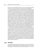
< ~P, where ~ can be calculated to be 0.034 for a 1 dB penalty using (5.12).
Since the generated FWM power increases with link length, this sets a limit on the
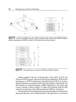
transmit power per channel as a function of the link length. This limit is plotted in
Figure 5.30 for both standard single-mode fiber (SMF) and dispersion-shifted fiber
(DSF) for three cases: (1) 8 channels spaced 100 GHz apart, (2) 32 channels spaced
100 GHz apart, and (3) 32 channels spaced 50 GHz apart. For SMF the chromatic
dispersion parameter is taken to be D = 17 ps/nm-km, and for DSF the chromatic
dispersion zero is assumed to lie in the middle of the transmitted band of channels.
The slope of the chromatic dispersion curve,
dD/d)~,
is taken to be
0.055
ps/nm-km 2.
We leave it as an exercise (Problem 5.27) to compute the power limits in the case of
NZ-DSF.
In Figure 5.30, first note that the limit is significantly worse in the case of
dispersion-shifted fiber than it is for standard fiber. This is because the four-wave
mixing efficiencies are much higher in dispersion-shifted fiber due to the low value
of the chromatic dispersion. Second, the power limit gets worse with an increas-
ing number of channels, as can be seen by comparing the limits for 8-channel and
32-channel systems for the same 100 GHz spacing. This effect is due to the much
larger number of four-wave mixing terms that are generated when the number of
channels is increased. In the case of dispersion-shifted fiber, this difference due to

the number of four-wave mixing terms is imperceptible since, even though there
are many more terms for the 32-channel case, the same 8 channels around the dis-
persion zero as in the 8-channel case contribute almost all the four-wave mixing
power. The four-wave mixing power contribution from the other channels is small
because there is much more chromatic dispersion at these wavelengths. Finally, the
power limit decreases significantly if the channel spacing is reduced, as can be seen
by comparing the curves for the two 32-channel systems with channel spacings of
100 GHz and 50 GHz. This decrease in the allowable transmit power arises because
the four-wave mixing efficiency increases with a decrease in the channel spacing
since the phase mismatch Aft is reduced. (For SMF, though the efficiencies at both
332 TRANSMISSION SYSTEM ENGINEERING
Figure
5.30 Limitation on the maximum transmit power per channel imposed by
four-wave mixing for systems operating over standard single-mode fiber and dispersion-
shifted fiber. For standard single-mode fiber, D is assumed to be 17 ps/nm-km, and for
dispersion-shifted fiber, the chromatic dispersion zero is assumed to lie in the middle of
the transmitted band of channels. The amplifiers are assumed to be spaced 80 km apart.
50 GHz and 100 GHz are small, the efficiency at 50 GHz is much higher than at
100 GHz.)
Four-wave mixing is a severe problem in WDM systems using dispersion-shifted
fiber but does not usually pose a major problem in systems using standard fiber. In
fact, it motivated the development of NZ-DSF fiber (see Section 5.7). In general, the
following actions alleviate the penalty due to four-wave mixing:
1. Unequal channel spacing: The positions of the channels can be chosen carefully
so that the beat terms do not overlap with the data channels inside the receiver
bandwidth. This may be possible for a small number of channels in some cases,
but needs careful computation of the exact channel positions.
2. Increased channel spacing: This increases the group velocity mismatch between
channels. This has the drawback of increasing the overall system bandwidth,
requiring the optical amplifiers to be flat over a wider bandwidth, and increases

the penalty due to SRS.
3. Using higher wavelengths beyond 1560 nm with DSF: Even with DSF, a signifi-
cant amount of chromatic dispersion is present in this range, which reduces the
5.8 Fiber Nonlinearities
333
effect of four-wave mixing. The newly developed L-band amplifiers can be used
for long-distance transmission over DSE
4. As with other nonlinearities, reducing transmitter power and the amplifier spac-
ing will decrease the penalty.
5. If the wavelengths can be demultiplexed and multiplexed in the middle of the
transmission path, we can introduce different delays for each wavelength. This
randomizes the phase relationship between the different wavelengths. Effectively,
the FWM powers introduced before and after this point are summed instead of
the electric fields being added in phase, resulting in a smaller FWM penalty.
5.8.5
Self-/Cross-Phase Modulation
As we saw in Section 2.4, SPM and CPM also arise out of the intensity dependence
of the refractive index. Fluctuations in optical power of the signal causes changes in
the phase of the signal. This induces additional chirp, which in turn, leads to higher
chromatic dispersion penalties. In practice, SPM can be a significant consideration in
designing systems at 10 Gb/s and higher, and leads to a restriction that the maximum
power per channel should not exceed a few milliwatts. CPM does not usually pose
a problem in WDM systems unless the channel spacings are extremely tight (a few
tens of gigahertz). In this section, we will study the system limitations imposed by
SPM.
The combined effects of SPM-induced chirp and dispersion can be studied by
numerically solving (E.15). For simplicity, we consider the following approximate
expression for the width TL of an initially unchirped Gaussian pulse after it has
propagated a distance L:
TL r Le L ( 4 L2e ) L2

~- 1 q 2 9 (5.27)
TO LNL LD 3~/~ LNL L 2
This expression is derived in [PAP86] starting from (E.15) and is also discussed in
[Agr95]. Note the similarity of this expression to the broadening factor for chirped
Gaussian pulses in (2.13);
Le/LNL
in (5.27) serves the role of the chirp factor in
(2.13).
Consider a 10 Gb/s system operating over standard single-mode fiber at 1.55 #m.
Since/32 < 0 and the SPM-induced chirp is positive, from Figure 2.11 we expect
that pulses will initially undergo compression and subsequently broaden. Since the
SPM-induced chirp increases with the transmitted power, we expect both the extent
of initial compression and the rate of subsequent broadening to increase with the
334
TRANSMISSION SYSTEM ENGINEERING
2-
1.8
1.6
1.4
~a 1.2
0.8
0.6
mW,.w 10
i I i , , i l
5~~____~~,'"'"'/ 1 O0 150 200 250
L (km)
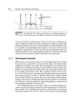
Figure
5.31 Evolution of pulse width as a function of the link length L for transmitted
powers of 1 mW, 10 mW, and 20 mW, taking into account the chirp induced by SPM.
A 10 Gb/s system operating over standard single-mode fiber at 1.55/zm with an initial

pulse width of 50 ps is considered.
transmitted power. This is indeed the case, as can be seen from Figure 5.31, where
we use (5.27) to plot the evolution of the pulse width as a function of the link length,
taking into account the chirp induced by SPM. We consider an initially unchirped
Gaussian pulse of width (half-width at 1/e-intensity point) 50 ps, which is half the
bit period. Three different transmitted powers, 1 mW, 10 mW, and 20 mW, are
considered. As expected, for a transmit power of 20 mW, the pulse compresses more
initially but subsequently broadens more rapidly so that the pulse width exceeds
that of a system operating at 10 mW or even 1 mW. The optimal transmit power
therefore depends on the link length and the amount of dispersion present. For
standard single-mode fiber in the 1.55/zm band, the optimal power is limited to the
2-10 mW range for link lengths on the order of 100 km and is a real limit today
for 10 Gb/s systems. We can use higher transmit powers to optimize other system
parameters such as the signal-to-noise ratio (SNR) but at the cost of increasing the
pulse broadening due to the combined effects of SPM and dispersion.
The system limits imposed by SPM can be calculated from (5.27) just as we did
in Figure 5.31. We can derive an expression for the power penalty due to SPM,
following the same approach as we did for chromatic dispersion. This is detailed in
Problem 5.25. Since SPM can be beneficial due to the initial pulse compression it can
cause, the SPM penalty can be negative. This occurs when the pulse at the end of the
link is narrower due to the chirping caused by SPM than it would be in the presence
of chromatic dispersion alone.
5.9 Wavelength Stabilization 335
5.8.6
In amplified systems, as we saw in Section 5.5, two things happen: the effective
length
L e
is multiplied by the number of amplifier spans as the amplifier resets the
power after each span, and in general, higher output powers are possible. Both of
these serve to exacerbate the effects of nonlinearities.

In WDM systems, CPM aids the SPM-induced intensity dependence of the re-
fractive index. Thus in WDM systems, these effects may become important even
at lower power levels, particularly when dispersion-shifted fiber is used so that the
dispersion-induced walk-off effects on CPM are minimized.
Role of Chromatic Dispersion Management
As we have seen, chromatic dispersion plays a key role in reducing the effects of non-
linearities, particularly four-wave mixing. However, chromatic dispersion by itself
produces penalties due to pulse smearing, which leads to intersymbol interference.
The important thing to note is that we can engineer systems with zero total chro-
matic dispersion but with chromatic dispersion present at all points along the link,
as shown in Figure 5.20. This approach leads to reduced penalties due to nonlinear-
ities, but the total chromatic dispersion is small so that we need not worry about
dispersion-induced penalties.
5.9
Wavelength Stabilization
Luckily for us, it turns out that the wavelength drift due to temperature variations
of some of the key components used in WDM systems is quite small. Typical mul-
tiplexers and demultiplexers made of silica/silicon have temperature coefficients of
0.01 nm/~ whereas DFB lasers have a temperature coefficient of 0.1 nm/~ Some
of the other devices that we studied in Chapter 3 have even lower temperature
coefficients.
The DFB laser source used in most systems is a key element that must be kept
wavelength stabilized. In practice, it may be sufficient to maintain the temperature of
the laser fairly constant to within +0.1 ~ which would stabilize the laser to within
4-0.01 nm/~ The laser comes packaged with a thermistor and a thermo-electric (TE)
cooler. The temperature can be sensed by monitoring the resistance of the thermistor
and can be kept constant by adjusting the drive current of the TE cooler. However,
the laser wavelength can also change because of aging effects over a long period.
Laser manufacturers usually specify this parameter, typically around +0.1 nm. If this
presents a problem, an external feedback loop may be required to stabilize the laser.

A small portion of the laser output can be tapped off and sent to a wavelength
discriminating element, such as an optical filter, called a
wavelength locker.
The
336 TRANSMISSION SYSTEM ENGINEERING
output of the wavelength locker can be monitored to establish the laser wavelength,
which can then be controlled by adjusting the laser temperature.
Depending on the temperature range needed (typically -10 to 60~ for equip-
ment in telco central offices), it may be necessary to temperature-control the
multiplexer/demultiplexer as well. For example, even if the multiplexer and de-
multiplexer are exactly aligned at, say, 25~ the ambient temperature at the two
ends of the link could be different by 70~ assuming the given numbers. Assuming a
temperature coefficient of 0.01 nm/~ we would get a 0.7 nm difference between the
center wavelengths of the multiplexer and demultiplexer, which is clearly intolerable
if the interchannel spacing is only 0.8 nm (100 GHz). One problem with tempera-
ture control is that it reduces the reliability of the overall component because the TE
cooler is often the least reliable component.
An additional factor to be considered is the dependence of laser wavelength on
its drive current, typically between 100 MHz/mA and i GHz/mA. A laser is typically
operated in one of two modes, constant output power or constant drive current, and
the drive circuitry incorporates feedback to maintain these parameters at constant
values. Keeping the drive current constant ensures that the laser wavelength does
not shift because of current changes. However, as the laser ages, it will require more
drive current to produce the same output power, so the output power may decrease
with time. On the other hand, keeping the power constant may require the drive
current to be increased as the laser ages, inducing a small wavelength shift. With
typical channel spacings of 100 GHz or thereabouts, this is not a problem, but with
tighter channel spacings, it may be desirable to operate the laser in constant current
mode and tolerate the penalty (if any) due to the reduced output power.
5.10

Design of Soliton Systems
While much of our discussion in this chapter applies to the design of soliton systems
as well, there are a few special considerations in the design of these systems, which
we now briefly discuss.
We discussed the fundamentals of soliton propagation in Section 2.5. Soliton
pulses balance the effects of chromatic dispersion and the nonlinear refractive index
of the fiber, to preserve their shapes during propagation. In order for this balance to
occur, the soliton pulses must not only have a specific shape but also a specific energy.
Due to the inevitable fiber attenuation, the pulse energies are reduced, and thus the
ideal soliton energy cannot be preserved. A theoretical solution to this problem is
the use of dispersion-tapered fibers, where the chromatic dispersion of the fiber is
varied suitably so that the balance between chromatic dispersion and nonlinearity is
preserved in the face of fiber loss.
5.10 Design of Soliton Systems
337
In practice, soliton propagation occurs reasonably well even in the case of systems
with periodic amplification. However, the ASE added by these amplifiers causes a few
detrimental effects. The first effect is that the ASE changes the energies of the pulses
and causes bit errors. This effect is similar to the effect in NRZ systems although the
quantitative details are somewhat different.
While solitons have a specific shape, they are resilient to changes in shape. For
example, if a pulse with a slightly different energy is launched, it reshapes itself into
a soliton component with the right shape and a nonsoliton component. When ASE
is added, the effect is to change the pulse shape, but the solitons reshape themselves
to the right shape.
A second effect of the ASE noise that is specific to soliton systems is that the
ASE noise causes random changes to the center frequencies of the soliton pulses. For
soliton propagation, per se, this would not be a problem because solitons can alter
their frequency without affecting their shape and energy. (This is the key to their
ability to propagate long distances without pulse spreading.) To see why this is the

case, consider the soliton pulse shape given by
U(~, r) =
ei~/2sechr.
(5.28)
Here, the distance ~ and time r are measured in terms of the chromatic dispersion
length of the fiber and the pulse width, respectively. The pulse
U(~, 75 + ~)e i(f2t+f22~/2
(5.29)
is also a soliton for any frequency shift Q, and thus solitons can alter their frequency
without affecting their shape and energy.
However, due to the chromatic dispersion of the fiber, changes in pulse frequencies
are converted into changes in the pulse arrival times, that is, timing jitter. This jitter
is called Gordon-Haus jitter, in honor of its discoverers, and is a significant problem
for soliton communication systems.
A potential solution to this timing jitter problem is the addition of a bandpass
filter whose center frequency is close to that of the launched soliton pulse. In the
presence of these filters, the solitons change their center frequencies to match the
passband of the filters. For this reason, these filters are called
guiding filters.
This has
the effect of keeping the soliton pulse frequencies stable, and hence minimizing the
timing jitter. This phenomenon is similar to the solitons reshaping themselves when
their shape is perturbed by the added ASE.
The problem with the above solution is that the ASE noise accumulates within
the passband of the chain of filters. As a result, the transmission length of the
system, before the timing jitter becomes unacceptable, is only moderately improved
compared to a system that does not use these filters. The solution to this problem
338
TRANSMISSION SYSTEM ENGINEERING
is to change the center frequencies of the filters progressively along the link length.

For example, if the filters are used every 20 km, each filter can be designed to have
a center frequency that is 0.2 GHz higher than the previous one. Over a distance
of 1000 km, this corresponds to a change of 10 GHz. The soliton pulses track the
center frequencies of the filters, but the accumulation of ASE noise is lessened. This
technique of using
sliding-frequency
guiding filters significantly minimizes timing
jitter and makes transoceanic soliton transmission practical.
5.11
Design of Dispersion-Managed Soliton Systems
There are a few drawbacks associated with conventional soliton systems. First, soli-
ton systems require fiber with a very low value of anomalous chromatic dispersion,
typically D < 0.2 ps/nm-km. This rules out the possibility of using solitons over the
existing fiber infrastructure, which primarily uses SMF or NZ-DSF, since these fibers
have much higher values of dispersion. Second, solitons require amplifier spacings
on the order of 20-25 kmmmuch closer than what is typically used in practical
WDM systems. Finally, cross-phase modulation (CPM) in WDM systems using con-
ventional solitons causes soliton-soliton collisions, resulting in timing jitter. For these
reasons, soliton systems have not been widely deployed.
The use of chirped RZ pulses (see Section 2.5.1), also called dispersion-managed
(DM) solitons, overcomes all three problems associated with soliton transmission.
First, these pulses can be used over a dispersion-managed fiber plant consisting of
fiber spans with large local chromatic dispersion, but with opposite signs such that
the total, or average, chromatic dispersion is small. This is typical of most fiber
plants used today for 10 Gb/s transmission since they consist of SMF or NZ-DSF
spans with dispersion compensation. Thus, no special fiber is required. Second, DM
solitons require amplification only every 60-80 km, which is compatible with the
amplifier spacings in today's WDM systems. Finally, the effect of CPM is vastly
reduced because of the large local chromatic dispersion and thus there is no timing
jitter problem. For the same reason, the Gordon-Haus jitter is also reduced, and

the sliding-frequency guiding filters used in conventional soliton systems are not
required.
In a dispersion-managed system, the spans between amplifiers consist of fibers
with alternating chromatic dispersions, as shown in Figure 5.32. Each fiber could
have a fairly high chromatic dispersion, but the total chromatic dispersion is small.
For example, each span in a dispersion-managed system could consist of a
50 km anomalous chromatic dispersion segment with a chromatic dispersion of
17 ps/nm-km, followed by a 30 km normal chromatic dispersion segment with a
chromatic dispersion of-25 ps/nm-km. The total chromatic dispersion over the
span is 50 x 17- 30 x 25 = 100 ps/km. The average chromatic dispersion is
5.11 Design of Dispersion-Managed Soliton Systems
339
Figure 5.32 A typical dispersion-managed span consisting of a segment of fiber
with anomalous chromatic dispersion followed by a segment with normal chromatic
dispersion.
100/80 = 1.25 ps/nm-km, which is anomalous. A dispersion-managed system could
have an average span dispersion that is normal or anomalous. In the same example,
if the normal fiber had a chromatic dispersion of -30 ps/nm-km, the average span
dispersion would have been -50/80 = -0.625 ps/nm-km, which is normal.
When NRZ pulses are used, the average chromatic dispersion can be anomalous
or normal, without having a significant impact on system performance. However,
in a DM soliton system, the average chromatic dispersion must be designed to be
anomalous in order to maintain the shape of the DM solitons. This is similar to
the case of conventional solitons, but with the crucial difference that the chromatic
dispersion need not be uniformly low and anomalous.
An important aspect of the design of DM soliton systems is the choice of the
peak transmit power and the average chromatic dispersion. Both should lie within
a certain range in order to achieve low BER operation. This range can be plotted as
a contour in a plot of peak transmit power versus average chromatic dispersion, as
shown in Figure 5.33. In this figure, we show a typical contour for achieving a BER

of 10 -~2 (or ~, = 7) in a 5160 km system with 80 km spans. For values ofthe transmit
power and average chromatic dispersion lying within this contour, the desired BER
is achieved or exceeded. In the same plot, the contour for a 2580 km NRZ system
with 80 km spans is also shown. In both NRZ and DM soliton systems, the allowed
transmit power has both a lower bound, determined by OSNR requirements, and an
upper bound determined by fiber nonlinear effects. From Figure 5.33, note that not
only is the DM soliton system capable of achieving regeneration-free transmission
for twice the distance as the NRZ system, it is also able to tolerate a much wider
range of variation in the transmit power and the average chromatic dispersion.