Handbook of mathematics for engineers and scienteists part 41 pot

248 LIMITS AND DERIVATIVES
3. Let f (x)beafunctiononafinite segment [a, b] satisfying the Lipschitz condition


f(x
1
)–f(x
2
)


≤ L|x
1
– x
2
|,
for any x
1
and x
2
in [a, b], where L is a constant. Then f(x) has bounded variation and
b
V
a
f(x) ≤ L(b – a).
4. Let f(x)beafunctiononafinite segment [a, b] with a bounded derivative |f

(x)| ≤ L,
where L = const. Then, f(x) is of bounded variation and
b
V

a
f(x) ≤ L(b – a).
5. Let f(x)beafunctionon[a, b]or[a, ∞) and suppose that f(x) can be represented
as an integral with variable upper limit,
f(x)=c +

x
a
ϕ(t) dt,
where ϕ(t) is an absolutely continuous function on the interval under consideration. Then
f(x) has bounded variation and
b
V
a
f(x)=

b
a
|ϕ(x)| dx.
C
OROLLARY.
Suppose that
ϕ(t)
on a finite segment
[a, b]
or
[a, ∞)
is integrable, but
not absolutely integrable. Then the total variation of
f(x)

is infinite.
6.1.7-3. Properties of functions of bounded variation.
Here, all functions are considered on a finite segment [a, b].
1. Any function of bounded variation is bounded.
2. The sum, difference, or product of finitely many functions of bounded variation is a
function of bounded variation.
3. Let f(x)andg(x) be two functions of bounded variation and |g(x)| ≥ K > 0.Then
the ratio f (x)/g(x) is a function of bounded variation.
4. Let a < c < b.Iff(x) has bounded variation on the segment [a, b], then it has bounded
variation on each segment [a, c]and[c, b]; and the converse statement is true. In this case,
the following additivity condition holds:
b
V
a
f(x)=
c
V
a
f(x)+
b
V
c
f(x).
5. Let f(x) be a function of bounded variation of the segment [a, b]. Then, for a ≤ x ≤ b,
the variation of f (x) with variable upper limit
F (x)=
x
V
a
f(x)

is a monotonically increasing bounded function of x.
6. Any function f (x) of bounded variation on the segment [a, b] has a left-hand limit
lim
x→x
0
–0
f(x) and a right-hand limit lim
x→x
0
+0
f(x) at any point x
0
[a, b].
6.1. BASIC CONCEPTS OF MAT H E M AT I CAL ANALYSIS 249
6.1.7-4. Criteria for functions to have bounded variation.
1. A function f(x) has bounded variation on a finite segment [a, b] if and only if there is
a monotonically increasing bounded function Φ(x) such that for all x
1
, x
2
[a, b](x
1
< x
2
),
the following inequality holds:
|f(x
2
)–f(x
1

)| ≤ Φ(x
2
)–Φ(x
1
).
2. A function f(x) has bounded variation on a finite segment [a, b] if and only if f(x)
can be represented as the difference of two monotonically increasing bounded functions on
that segment: f(x)=g
2
(x)–g
1
(x).
Remark. The above criteria are valid also for infinite intervals (–∞, a], [a, ∞), and (–∞, ∞).
6.1.7-5. Properties of continuous functions of bounded variation.
1. Let f(x) be a function of bounded variation on the segment [a, b]. If f (x)is
continuous at a point x
0
(a < x
0
< b), then the function F (x)=
x
V
a
f(x) is also continuous
at that point.
2. A continuous function of bounded variation can be represented as the difference of
two continuous increasing functions.
3. Let f(x) be a continuous function on the segment [a, b]. Consider a partition of the
segment
a = x

0
< x
1
< x
2
< ··· < x
n–1
< x
n
= b
and the sum v =
n–1

k=0


f(x
k+1
)–f(x
k
)


. Letting λ =max|x
k+1
– x
k
| and passing to the limit
as λ → 0,weget
lim

λ→0
v =
b
V
a
f(x).
6.1.8. Convergence of Functions
6.1.8-1. Pointwise, uniform, and nonuniform convergence of functions.
Let {f
n
(x)} be a sequence of functions defined on a set X ⊂R. The sequence {f
n
(x)} is said
to be pointwise convergent to f(x)asn →∞if for any fixed x X, the numerical sequence
{f
n
(x)} converges to f(x). The sequence {f
n
(x)} is said to be uniformly convergent to a
function f(x)onX as n →∞if for any ε > 0 there is an integer N = N(ε) and such that
for all n > N and all x
X, the following inequality holds:
|f
n
(x)–f(x)| < ε.(6.1.8.1)
Note that in this definition, N is independent of x. For a sequence {f
n
(x)} pointwise
convergent to f (x)asn →∞,bydefinition, for any ε > 0 and any x X,thereis
N = N(ε, x) such that (6.1.8.1) holds for all n > N(ε, x). If one cannot find such N

independent of x and depending only on ε (i.e., one cannot ensure (6.1.8.1) uniformly; to be
more precise, there is δ > 0 such that for any N > 0 there is k
N
> N and x
N
X such that
|f
k
N
(x
N
)–f(x
N
)| ≥ δ), then one says that the sequence {f
n
(x)} converges nonuniformly
to f(x)onthesetX.
250 LIMITS AND DERIVATIVES
6.1.8-2. Basic theorems.
Let X be an interval on the real axis.
T
HEOREM.
Let
f
n
(x)
be a sequence of continuous functions uniformly convergent to
f(x)
on
X

.Then
f(x)
is continuous on
X
.
COROLLARY.
If the limit function
f(x)
of a pointwise convergent sequence of contin-
uous functions
{f
n
(x)}
is discontinuous, then the convergence of the sequence
{f
n
(x)}
is
nonuniform.
Example. The sequence {f
n
(x)} = {x
n
} converges to f (x) ≡ 0 as n →∞uniformly on each segment
[0, a], 0 < a < 1. However, on the segment [0, 1] this sequence converges nonuniformly to the discontinuous
function f(x)=

0 for 0 ≤ x < 1,
1 for x = 1.
CAUCHY CRITERION.

A sequence of functions
{f
n
(x)}
defined on a set
X R
uniformly
converges to
f(x)
as
n →∞
if and only if for any
ε > 0
there is an integer
N = N(ε)>0
such that for all
n > N
and
m > N
, the inequality
|f
n
(x)–f
m
(x)| < ε
holds for all
x X
.
6.1.8-3. Geometrical meaning of uniform convergence.
Let f

n
(x) be continuous functions on the segment [a, b] and suppose that {f
n
(x)} uniformly
converges to a continuous function f(x)asn →∞. Then all curves y =f
n
(x), for sufficiently
large n > N , belong to the strip between the two curves y = f (x)–ε and y = f(x)+ε (see
Fig. 6.3).
O
x
y
ba
yfx= ()
yfx= ()+ε
yfx=-() ε
yfx= ()
n
Figure 6.3. Geometrical meaning of uniform convergence of a sequence of functions {f
n
(x)} to a continuous
function f (x).
6.2. Differential Calculus for Functions of a Single
Variable
6.2.1. Derivative and Differential, Their Geometrical and Physical
Meaning
6.2.1-1. Definition of derivative and differential.
The derivative of a function y = f(x) at a point x is the limit of the ratio
y


= lim
Δx→0
Δy
Δx
= lim
Δx→0
f(x + Δx)–f (x)
Δx
,
where Δy = f(x+Δx)–f(x) is the increment of the function corresponding to the increment
of the argument Δx. The derivative y

is also denoted by y

x
, ˙y,
dy
dx
, f

(x),
df (x)
dx
.
6.2. DIFFERENTIAL CALCULUS FOR FUNCTIONS OF A SINGLE VARIABLE 251
Example 1. Let us calculate the derivative of the function f(x)=x
2
.
By definition, we have
f


(x) = lim
Δx→0
(x + Δx)
2
– x
2
Δx
= lim
Δx→0
(2x + Δx)=2x.
The increment Δx is also called the differential of the independent variable x and is
denoted by dx.
A function f (x) that has a derivative at a point x is called differentiable at that point.
The differentiability of f (x) at a point x is equivalent to the condition that the increment
of the function, Δy = f(x + dx)–f(x), at that point can be represented in the form
Δy = f

(x) dx + o(dx) (the second term is an infinitely small quantity compared with dx as
dx → 0).
A function differentiable at some point x is continuous at that point. The converse is
not true, in general; continuity does not always imply differentiability.
A function f (x) is called differentiable on a set D (interval, segment, etc.) if for any
x
D there exists the derivative f

(x). A function f(x) is called continuously differentiable
on D if it has the derivative f

(x) at each point x D and f


(x) is a continuous function on
D.
The differential dy of a function y = f(x) is the principal part of its increment Δy at the
point x,sothat dy = f

(x)dx, Δy = dy + o(dx).
The approximate relation Δy ≈ dy or f (x + Δx) ≈ f(x)+f

(x)Δx (for small Δx)is
often used in numerical analysis.
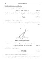
6.2.1-2. Physical and geometrical meaning of the derivative. Tangent line.
1
◦
.Lety = f(x) be the function describing the path y traversed by a body by the time x.
Then the derivative f

(x) is the velocity of the body at the instant x.
2
◦
.Thetangent line or simply the tangent to the graph of the function y = f (x) at a point
M(x
0
, y
0
), where y
0
= f(x
0
), is defined as the straight line determined by the limit position

of the secant MN as the point N tends to M along the graph. If α is the angle between
the x-axis and the tangent line, then f

(x
0
)=tanα is the slope ratio of the tangential line
(Fig. 6.4).
O
x
y
y
dy
M
N
α
α
Δy
0
yfx= ()
x
0
x+ xΔ
0
Figure 6.4. The tangent to the graph of a function y = f(x) at a point (x
0
, y
0
).
Equation of the tangent line to the graph of a function y = f (x) at a point (x
0

, y
0
):
y – y
0
= f

(x
0
)(x – x
0
).
252 LIMITS AND DERIVATIVES
Equation of the normal to the graph of a function y = f(x) at a point (x
0
, y
0
):
y – y
0
=–
1
f

(x
0
)
(x – x
0
).

6.2.1-3. One-sided derivatives.
One-sided derivatives are defined as follows:
f

+
(x) = lim
Δx→+0
Δy
Δx
= lim
Δx→+0
f(x + Δx)–f (x)
Δx
right-hand derivative,
f

–
(x) = lim
Δx→–0
Δy
Δx
= lim
Δx→–0
f(x + Δx)–f(x)
Δx
left-hand derivative.
Example 2. The function y = |x| at the point x = 0 has different one-sided derivatives: y

+
(0)=1, y


–
(0)=–1,
but has no derivative at that point. Such points are called angular points.
Suppose that a function y = f(x) is continuous at x = x
0
and has equal one-sided
derivatives at that point, y

+
(x
0
)=y

–
(x
0
)=a. Then this function has a derivative at x = x
0
and y

(x
0
)=a.
6.2.2. Table of Derivatives and Differentiation Rules
The derivative of any elementary function can be calculated with the help of derivatives of
basic elementary functions and differentiation rules.
6.2.2-1. Table of derivatives of basic elementary functions (a = const).
(a)


= 0,(x
a
)

= ax
a–1
,
(e
x
)

= e
x
,(a
x
)

= a
x
ln a,
(ln x)

=
1
x
,(log
a
x)

=

1
x ln a
,
(sin x)

=cosx,(cosx)

=–sinx,
(tan x)

=
1
cos
2
x
,(cotx)

=–
1
sin
2
x
,
(arcsin x)

=
1
√
1 – x
2

, (arccos x)

=–
1
√
1 – x
2
,
(arctan x)

=
1
1 + x
2
, (arccot x)

=–
1
1 + x
2
,
(sinh x)

=coshx,(coshx)

=sinhx,
(tanh x)

=
1

cosh
2
x
,(cothx)

=–
1
sinh
2
x
,
(arcsinh x)

=
1
√
1 + x
2
, (arccosh x)

=
1
√
x
2
– 1
,
(arctanh x)

=

1
1 – x
2
, (arccoth x)

=
1
x
2
– 1
.
6.2. DIFFERENTIAL CALCULUS FOR FUNCTIONS OF A SINGLE VARIABLE 253
6.2.2-2. Differentiation rules.
1. Derivative of a sum (difference) of functions:
[u(x)
v(x)]

= u

(x) v

(x).
2. Derivative of the product of a function and a constant:
[au(x)]

= au

(x)(a = const).
3. Derivative of a product of functions:
[u(x)v(x)]


= u

(x)v(x)+u(x)v

(x).
4. Derivative of a ratio of functions:

u(x)
v(x)


=
u

(x)v(x)–u(x)v

(x)
v
2
(x)
.
5. Derivative of a composite function:

f(u(x))


= f

u

(u)u

(x).
6. Derivative of a parametrically defined function x = x(t), y = y(t):
y

x
=
y

t
x

t
.
7. Derivative of an implicit function defined by the equation F (x, y)=0:
y

x
=–
F
x
F
y
(F
x
and F
y
are partial derivatives).
8. Derivative of the inverse function x = x(y) (for details see footnote*):

x

y
=
1
y

x
.
9. Derivative of a composite exponential function:
[u(x)
v(x)
]

= u
v
ln u ⋅ v

+ vu
v–1
u

.
10. Derivative of a composite function of two arguments:
[f(u(x), v(x))]

= f
u
(u, v)u


+ f
v
(u, v)v

(f
u
and f
v
are partial derivatives).
Example 1. Let us calculate the derivative of the function
x
2
2x + 1
.
Using the rule of differentiating the ratio of two functions, we obtain

x
2
2x + 1


=
(x
2
)

(2x + 1)–x
2
(2x + 1)


(2x + 1)
2
=
2x(2x + 1)–2x
2
(2x + 1)
2
=
2x
2
+ 2x
(2x + 1)
2
.
Example 2. Let us calculate the derivative of the function ln cos x.
Using the rule of differentiating composite functions and the formula for the logarithmic derivative from
Paragraph 6.2.2-1, we get
(ln cos x)

=
1
cos x
(cos x)

=–tanx.
Example 3. Let us calculate the derivative of the function x
x
. Using the rule of differentiating the
composite exponential function with u(x)=v(x)=x,wehave
(x

x
)

= x
x
ln x + xx
x–1
= x
x
(ln x + 1).
*Lety = f(x) be a differentiable monotone function on the interval (a, b)andf

(x
0
) ≠ 0,wherex
0
(a, b).
Then the inverse function x = g(y) is differentiable at the point y
0
= f(x
0
)and g

(y
0
)=
1
f

(x

0
)
.
254 LIMITS AND DERIVATIVES
6.2.3. Theorems about Differentiable Functions. L’Hospital Rule
6.2.3-1. Main theorems about differentiable functions.
ROLLE THEOREM.
If the function
y = f(x)
is continuous on the segment
[a, b]
,differ-
entiable on the interval
(a, b)
,and
f(a)=f (b)
, then there is a point
c (a, b)
such that
f

(c)=0
.
LAGRANGE THEOREM.
If the function
y = f (x)
is continuous on the segment
[a, b]
and
differentiable on the interval

(a, b)
, then there is a point
c (a, b)
such that
f(b)–f(a)=f

(c)(b – a).
This relation is called the formula of finite increments.
C
AUCHY THEOREM.
Let
f(x)
and
g(x)
be two functions that are continuous on the
segment
[a, b]
, differentiable on the interval
(a, b)
,and
g

(x) ≠ 0
for all
x (a, b)
.Then
there is a point
c (a, b)
such that
f(b)–f(a)

g(b)–g(a)
=
f

(c)
g

(c)
.
6.2.3-2. L’Hospital’s rules on indeterminate expressions of the form 0/0 and ∞ /∞.
THEOREM 1.
Let
f(x)
and
g(x)
be two functions defined in a neighborhood of a point
a
, vanishing at this point,
f(a)=g(a)=0
, and having the derivatives
f

(a)
and
g

(a)
, with
g


(a) ≠ 0
.Then
lim
x→a
f(x)
g(x)
=
f

(a)
g

(a)
.
Example 1. Let us calculate the limit lim
x→0
sin x
1 – e
–2x
.
Here, both the numerator and the denominator vanish for x = 0. Let us calculate the derivatives
f

(x)=(sinx)

=cosx =⇒ f

(0)=1,
g


(x)=(1 – e
–2x
)

= 2e
–2x
=⇒ g

(0)=2 ≠ 0.
By the L’Hospital rule, we find that
lim
x→0
sin x
1 – e
–2x
=
f

(0)
g

(0)
=
1
2
.
THEOREM 2.
Let
f(x)
and

g(x)
be two functions defined in a neighborhood of a point
a
, vanishing at
a
, together with their derivatives up to the order
n – 1
inclusively. Suppose
also that the derivatives
f
(n)
(a)
and
g
(n)
(a)
exist and are finite,
g
(n)
(a) ≠ 0
.Then
lim
x→a
f(x)
g(x)
=
f
(n)
(a)
g

(n)
(a)
.
T
HEOREM 3.
Let
f(x)
and
g(x)
be differentiable functions and
g

(x) ≠ 0
in a neighbor-
hood of a point
a
(
x ≠ a
). If
f(x)
and
g(x)
are infinitely small or infinitely large functions
for
x → a
, i.e., the ratio
f(x)
g(x)
at the point
a

is an indeterminate expression of the form
0
0
or
∞
∞
,then
lim
x→a
f(x)
g(x)
= lim
x→a
f

(x)
g

(x)
(provided that there exists a finite or infinite limit of the ratio of the derivatives).
Remark. The L’Hospital rule 3 is applicable also in the case of a being one of the symbols ∞,+∞,–∞.