SAS/ETS 9.22 User''''s Guide 87 docx

852 ✦ Chapter 15: The FORECAST Procedure
OUTEST= Data Set
The FORECAST procedure writes the parameter estimates and goodness-of-fit statistics to an output
data set when the OUTEST= option is specified. The OUTEST= data set contains the following
variables:
 the BY variables

the first ID variable, which contains the value of the ID variable for the last observation in the
input data set used to fit the model
 _TYPE_, a character variable that identifies the type of each observation

the VAR statement variables, which contain statistics and parameter estimates for the input
series. The values contained in the VAR statement variables depend on the _TYPE_ variable
value for the observation.
The observations contained in the OUTEST= data set are identified by the _TYPE_ variable. The
OUTEST= data set might contain observations with the following _TYPE_ values:
AR1–ARn
The observation contains estimates of the autoregressive parameters for the series.
Two-digit lag numbers are used if the value of the NLAGS= option is 10 or more;
in that case these _TYPE_ values are AR01–ARn. These observations are output
for the STEPAR method only.
CONSTANT
The observation contains the estimate of the constant or intercept parameter
for the time trend model for the series. For the exponential smoothing and the
Winters’ methods, the trend model is centered (that is, t =0) at the last observation
used for the fit.
LINEAR
The observation contains the estimate of the linear or slope parameter for the
time trend model for the series. This observation is output only if you specify
TREND=2 or TREND=3.
N

The observation contains the number of nonmissing observations used to fit the
model for the series.
QUAD
The observation contains the estimate of the quadratic parameter for the time trend
model for the series. This observation is output only if you specify TREND=3.
SIGMA
The observation contains the estimate of the standard deviation of the error term
for the series.
S1–S3
The observations contain exponentially smoothed values at the last observa-
tion. _TYPE_=S1 is the final smoothed value of the single exponential smooth.
_TYPE_=S2 is the final smoothed value of the double exponential smooth.
_TYPE_=S3 is the final smoothed value of the triple exponential smooth. These
observations are output for METHOD=EXPO only.
OUTEST= Data Set ✦ 853
S_name
The observation contains estimates of the seasonal parameters. For example,
if SEASONS=MONTH, the OUTEST= data set contains observations with
_TYPE_=S_JAN, _TYPE_=S_FEB, _TYPE_=S_MAR, and so forth.
For multiple-period seasons, the names of the first and last interval of the season
are concatenated to form the season name. Thus, for SEASONS=MONTH4,
the OUTEST= data set contains observations with _TYPE_=S_JANAPR,
_TYPE_=S_MAYAUG, and _TYPE_=S_SEPDEC.
When the SEASONS= option specifies numbers, the seasonal factors are labeled
_TYPE_=S_i_j. For example, SEASONS=(2 3) produces observations with
_TYPE_ values of S_1_1, S_1_2, S_2_1, S_2_2, and S_2_3. The observation
with _TYPE_=S_i_j contains the seasonal parameters for the jth season of the ith
seasonal cycle.
These observations are output only for METHOD=WINTERS or
METHOD=ADDWINTERS.

WEIGHT
The observation contains the smoothing weight used for exponential smooth-
ing. This is the value of the WEIGHT= option. This observation is output for
METHOD=EXPO only.
WEIGHT1
WEIGHT2
WEIGHT3
The observations contain the weights used for smoothing the WINTERS
or ADDWINTERS method parameters (specified by the WEIGHT= option).
_TYPE_=WEIGHT1 is the weight used to smooth the CONSTANT parameter.
_TYPE_=WEIGHT2 is the weight used to smooth the LINEAR and QUAD
parameters. _TYPE_=WEIGHT3 is the weight used to smooth the seasonal
parameters. These observations are output only for the WINTERS and ADDWIN-
TERS methods.
NRESID
The observation contains the number of nonmissing residuals, n, used to compute
the goodness-of-fit statistics. The residuals are obtained by subtracting the one-
step-ahead predicted values from the observed values.
SST
The observation contains the total sum of squares for the series, corrected for the
mean. SST D
P
n
tD1
.y
t
 y/
2
, where y is the series mean.
SSE

The observation contains the sum of the squared residuals, uncorrected for the
mean.
SSE D
P
n
tD1
.y
t
 Oy
t
/
2
, where
Oy
is the one-step predicted value for the
series.
MSE
The observation contains the mean squared error, calculated from one-step-ahead
forecasts.
MSE D
1
nk
SSE
, where k is the number of parameters in the model.
RMSE The observation contains the root mean squared error. RMSE D
p
MSE.
MAPE The observation contains the mean absolute percent error.
MAPE D
100

n
P
n
tD1
j.y
t
 Oy
t
/=y
t
j.
MPE The observation contains the mean percent error.
MPE D
100
n
P
n
tD1
.y
t
 Oy
t
/=y
t
.
MAE The observation contains the mean absolute error. MAE D
1
n
P
n

tD1
jy
t
 Oy
t
j.
854 ✦ Chapter 15: The FORECAST Procedure
ME The observation contains the mean error. MAE D
1
n
P
n
tD1
.y
t
 Oy
t
/.
MAXE The observation contains the maximum error (the largest residual).
MINE The observation contains the minimum error (the smallest residual).
MAXPE The observation contains the maximum percent error.
MINPE The observation contains the minimum percent error.
RSQUARE
The observation contains the R square statistic,
R
2
D 1  SSE=SS T
. If the
model fits the series badly, the model error sum of squares SSE might be larger
than SST and the R square statistic will be negative.

ADJRSQ The observation contains the adjusted R square statistic.
ADJRSQ D 1  .
n1
nk
/.1  R
2
/.
ARSQ The observation contains Amemiya’s adjusted R square statistic.
ARSQ D 1  .
nCk
nk
/.1  R
2
/.
RW_RSQ
The observation contains the random walk R square statistic (Harvey’s
R
2
D
statistic
that uses the random walk model for comparison).
RW _RSQ D 1  .
n1
n
/SSE=RW SSE,
where RW SSE D
P
n
tD2
.y

t
 y
t1
 /
2
and  D
1
n1
P
n
tD2
.y
t
 y
t1
/.
AIC The observation contains Akaike’s information criterion.
AIC D nln.SSE=n/ C 2k.
SBC The observation contains Schwarz’s Bayesian criterion.
SBC D nln.S SE=n/ C kln.n/.
APC The observation contains Amemiya’s prediction criterion.
AP C D
1
n
SST .
nCk
nk
/.1  R
2
/ D .

nCk
nk
/
1
n
SSE.
CORR
The observation contains the correlation coefficient between the actual values and
the one-step-ahead predicted values.
THEILU
The observation contains Theil’s U statistic that uses original units. See Maddala
(1977, pp. 344–345), and Pindyck and Rubinfeld (1981, pp. 364–365) for more
information about Theil statistics.
RTHEILU The observation contains Theil’s U statistic calculated using relative changes.
THEILUM The observation contains the bias proportion of Theil’s U statistic.
THEILUS The observation contains the variance proportion of Theil’s U statistic.
THEILUC The observation contains the covariance proportion of Theil’s U statistic.
THEILUR The observation contains the regression proportion of Theil’s U statistic.
THEILUD The observation contains the disturbance proportion of Theil’s U statistic.
RTHEILUM
The observation contains the bias proportion of Theil’s U statistic, calculated by
using relative changes.
RTHEILUS
The observation contains the variance proportion of Theil’s U statistic, calculated
by using relative changes.
Examples: FORECAST Procedure ✦ 855
RTHEILUC
The observation contains the covariance proportion of Theil’s U statistic, calcu-
lated by using relative changes.
RTHEILUR

The observation contains the regression proportion of Theil’s U statistic, calcu-
lated by using relative changes.
RTHEILUD
The observation contains the disturbance proportion of Theil’s U statistic, calcu-
lated by using relative changes.
Examples: FORECAST Procedure
Example 15.1: Forecasting Auto Sales
This example uses the Winters method to forecast the monthly U. S. sales of passenger cars series
(VEHICLES) from the data set SASHELP.USECON. These data are taken from Business Statistics,
published by the U. S. Bureau of Economic Analysis.
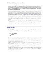
The following statements plot the series. The plot is shown in Output 15.1.1.
title1 "Sales of Passenger Cars";
symbol1 i=spline v=dot;
axis2 label=(a=-90 r=90 "Vehicles and Parts" )
order=(6000 to 24000 by 3000);
title1 "Sales of Passenger Cars";
proc sgplot data=sashelp.usecon;
series x=date y=vehicles / markers;
xaxis values=('1jan80'd to '1jan92'd by year);
yaxis values=(6000 to 24000 by 3000);
format date year4.;
run;
856 ✦ Chapter 15: The FORECAST Procedure
Output 15.1.1 Monthly Passenger Car Sales
The following statements produce the forecast:
proc forecast data=sashelp.usecon interval=month
method=winters seasons=month lead=12
out=out outfull outresid outest=est;
id date;
var vehicles;

where date >= '1jan80'd;
run;
The INTERVAL=MONTH option indicates that the data are monthly, and the ID DATE statement
gives the dating variable. The METHOD=WINTERS specifies the Winters smoothing method. The
LEAD=12 option forecasts 12 months ahead. The OUT=OUT option specifies the output data set,
while the OUTFULL and OUTRESID options include in the OUT= data set the predicted and residual
values for the historical period and the confidence limits for the forecast period. The OUTEST=
option stores various statistics in an output data set. The WHERE statement is used to include only
data from 1980 on.
The following statements print the OUT= data set (first 20 observations):
proc print data=out (obs=20) noobs;
run;
Example 15.1: Forecasting Auto Sales ✦ 857
The listing of the output data set produced by PROC PRINT is shown in part in Output 15.1.2.
Output 15.1.2 The OUT= Data Set Produced by PROC FORECAST (First 20 Observations)
Sales of Passenger Cars
DATE _TYPE_ _LEAD_ VEHICLES
JAN80 ACTUAL 0 8808.00
JAN80 FORECAST 0 8046.52
JAN80 RESIDUAL 0 761.48
FEB80 ACTUAL 0 10054.00
FEB80 FORECAST 0 9284.31
FEB80 RESIDUAL 0 769.69
MAR80 ACTUAL 0 9921.00
MAR80 FORECAST 0 10077.33
MAR80 RESIDUAL 0 -156.33
APR80 ACTUAL 0 8850.00
APR80 FORECAST 0 9737.21
APR80 RESIDUAL 0 -887.21
MAY80 ACTUAL 0 7780.00

MAY80 FORECAST 0 9335.24
MAY80 RESIDUAL 0 -1555.24
JUN80 ACTUAL 0 7856.00
JUN80 FORECAST 0 9597.50
JUN80 RESIDUAL 0 -1741.50
JUL80 ACTUAL 0 6102.00
JUL80 FORECAST 0 6833.16
The following statements print the OUTEST= data set:
title2 'The OUTEST= Data Set: WINTERS Method';
proc print data=est;
run;
The PROC PRINT listing of the OUTEST= data set is shown in Output 15.1.3.
858 ✦ Chapter 15: The FORECAST Procedure
Output 15.1.3 The OUTEST= Data Set Produced by PROC FORECAST
Sales of Passenger Cars
The OUTEST= Data Set: WINTERS Method
Obs _TYPE_ DATE VEHICLES
1 N DEC91 144
2 NRESID DEC91 144
3 DF DEC91 130
4 WEIGHT1 DEC91 0.1055728
5 WEIGHT2 DEC91 0.1055728
6 WEIGHT3 DEC91 0.25
7 SIGMA DEC91 1741.481
8 CONSTANT DEC91 18577.368
9 LINEAR DEC91 4.804732
10 S_JAN DEC91 0.8909173
11 S_FEB DEC91 1.0500278
12 S_MAR DEC91 1.0546539
13 S_APR DEC91 1.074955

14 S_MAY DEC91 1.1166121
15 S_JUN DEC91 1.1012972
16 S_JUL DEC91 0.7418297
17 S_AUG DEC91 0.9633888
18 S_SEP DEC91 1.051159
19 S_OCT DEC91 1.1399126
20 S_NOV DEC91 1.0132126
21 S_DEC DEC91 0.802034
22 SST DEC91 2.63312E9
23 SSE DEC91 394258270
24 MSE DEC91 3032755.9
25 RMSE DEC91 1741.481
26 MAPE DEC91 9.4800217
27 MPE DEC91 -1.049956
28 MAE DEC91 1306.8534
29 ME DEC91 -42.95376
30 RSQUARE DEC91 0.8502696
The following statements plot the residuals. The plot is shown in Output 15.1.4.
title1 "Sales of Passenger Cars";
title2 'Plot of Residuals';
proc sgplot data=out;
where _type_ = 'RESIDUAL';
needle x=date y=vehicles / markers markerattrs=(symbol=circlefilled);
xaxis values=('1jan80'd to '1jan92'd by year);
format date year4.;
run;
Example 15.1: Forecasting Auto Sales ✦ 859
Output 15.1.4 Residuals from Winters Method
The following statements plot the forecast and confidence limits. The last two years of historical
data are included in the plot to provide context for the forecast plot. A reference line is drawn at the

start of the forecast period.
title1 "Sales of Passenger Cars";
title2 'Plot of Forecast from WINTERS Method';
proc sgplot data=out;
series x=date y=vehicles / group=_type_ lineattrs=(pattern=1);
where _type_ ^= 'RESIDUAL';
refline '15dec91'd / axis=x;
yaxis values=(9000 to 25000 by 1000);
xaxis values=('1jan90'd to '1jan93'd by qtr);
run;
The plot is shown in Output 15.1.5.
860 ✦ Chapter 15: The FORECAST Procedure
Output 15.1.5 Forecast of Passenger Car Sales
Example 15.2: Forecasting Retail Sales
This example uses the stepwise autoregressive method to forecast the monthly U. S. sales of durable
goods (DURABLES) and nondurable goods (NONDUR) from the SASHELP.USECON data set.
The data are from Business Statistics, published by the U.S. Bureau of Economic Analysis. The
following statements plot the series:
title1 'Sales of Durable and Nondurable Goods';
title2 'Plot of Forecast from WINTERS Method';
proc sgplot data=sashelp.usecon;
series x=date y=durables / markers markerattrs=(symbol=circlefilled);
xaxis values=('1jan80'd to '1jan92'd by year);
yaxis values=(60000 to 150000 by 10000);
format date year4.;
run;
Example 15.2: Forecasting Retail Sales ✦ 861
title1 'Sales of Durable and Nondurable Goods';
title2 'Plot of Forecast from WINTERS Method';
proc sgplot data=sashelp.usecon;

series x=date y=nondur / markers markerattrs=(symbol=circlefilled);
xaxis values=('1jan80'd to '1jan92'd by year);
yaxis values=(70000 to 130000 by 10000);
format date year4.;
run;
The plots are shown in Output 15.2.1 and Output 15.2.2.
Output 15.2.1 Durable Goods Sales