SAS/ETS 9.22 User''''s Guide 121 ppsx

1192 ✦ Chapter 18: The MODEL Procedure
If k is the number of general form equations, then k derivatives are required.
The convergence properties of the Jacobi and Seidel solution methods remain significantly poorer
than the default Newton’s method.
Comparison of Methods
Newton’s method is the default and should work better than the others for most small- to medium-
sized models. The Seidel method is always faster than the Jacobi for recursive models with equations
in recursive order. For very large models and some highly nonlinear smaller models, the Jacobi or
Seidel methods can sometimes be faster. Newton’s method uses more memory than the Jacobi or
Seidel methods.
Both the Newton’s method and the Jacobi method are order-invariant in the sense that the order in
which equations are specified in the model program has no effect on the operation of the iterative
solution process. In order-invariant methods, the values of the solution variables are fixed for the
entire execution of the model program. Assignments to model variables are automatically changed
to assignments to corresponding equation variables. Only after the model program has completed
execution are the results used to compute the new solution values for the next iteration.
Troubleshooting Problems
In solving a simultaneous nonlinear dynamic model you might encounter some of the following
problems.
Missing Values
For SOLVE tasks, there can be no missing parameter values. Missing right-hand-side variables result
in missing left-hand-side variables for that observation.
Unstable Solutions
A solution might exist but be unstable. An unstable system can cause the Jacobi and Seidel methods
to diverge.
Explosive Dynamic Systems
A model might have well-behaved solutions at each observation but be dynamically unstable. The
solution might oscillate wildly or grow rapidly with time.
Propagation of Errors
During the solution process, solution variables can take on values that cause computational errors.
For example, a solution variable that appears in a LOG function might be positive at the solution

but might be given a negative value during one of the iterations. When computational errors occur,
missing values are generated and propagated, and the solution process might collapse.
Numerical Solution Methods ✦ 1193
Convergence Problems
The following items can cause convergence problems:
 There are illegal function values ( for example
p
1 ).
 There are local minima in the model equation.
 No solution exists.
 Multiple solutions exist.
 Initial values are too far from the solution.
 The CONVERGE= value is too small.
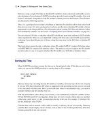
When PROC MODEL fails to find a solution to the system, the current iteration information and
the program data vector are printed. The simulation halts if actual values are not available for
the simulation to proceed. Consider the following program, which produces the output shown in
Figure 18.82:
data test1;
do t=1 to 50;
x1 = sqrt(t) ;
y = .;
output;
end;
proc model data=test1;
exogenous x1 ;
control a1 -1 b1 -29 c1 -4 ;
y = a1
*
sqrt(y) + b1
*

x1
*
x1 + c1
*
lag(x1);
solve y / out=sim forecast dynamic ;
run;
Figure 18.82 SOLVE Convergence Problems
The MODEL Procedure
Dynamic Single-Equation Forecast
ERROR: Could not reduce norm of residuals in 10 subiterations.
ERROR: The solution failed because 1 equations are missing or have extreme
values for observation 1 at NEWTON iteration 1.
NOTE: Additional information on the values of the variables at this
observation, which may be helpful in determining the cause of the failure
of the solution process, is printed below.
Observation 1 Iteration 1 CC -1.000000
Missing 1
Iteration Errors - Missing.
1194 ✦ Chapter 18: The MODEL Procedure
Figure 18.82 continued
The MODEL Procedure
Dynamic Single-Equation Forecast
Listing of Program Data Vector
_N_: 12 ACTUAL.x1: 1.41421 ACTUAL.y: .
ERROR.y: . PRED.y: . a1: -1
b1: -29 c1: -4 x1: 1.41421
y: -0.00109
@PRED.y/@y: . @ERROR.y/@y: .
NOTE: Check for missing input data or uninitialized lags.

(Note that the LAG and DIF functions return missing values for the
initial lag starting observations. This is a change from the 1982 and earlier
versions of SAS/ETS which returned zero for uninitialized lags.)
NOTE: Simulation aborted.
At the first observation, a solution to the following equation is attempted:
y D 
p
y 62
There is no solution to this problem. The iterative solution process got as close as it could to making
Y negative while still being able to evaluate the model. This problem can be avoided in this case by
altering the equation.
In other models, the problem of missing values can be avoided by either altering the data set to
provide better starting values for the solution variables or by altering the equations.
You should be aware that, in general, a nonlinear system can have any number of solutions and the
solution found might not be the one that you want. When multiple solutions exist, the solution that is
found is usually determined by the starting values for the iterations. If the value from the input data
set for a solution variable is missing, the starting value for it is taken from the solution of the last
period (if nonmissing) or else the solution estimate is started at 0.
Iteration Output
The iteration output, produced by the ITPRINT option, is useful in determining the cause of a
convergence problem. The ITPRINT option forces the printing of the solution approximation and
equation errors at each iteration for each observation. A portion of the ITPRINT output from the
following statements is shown in Figure 18.83.
proc model data=test1;
exogenous x1 ;
control a1 -1 b1 -29 c1 -4 ;
y = a1
*
sqrt(abs(y)) + b1
*

x1
*
x1 + c1
*
lag(x1);
solve y / out=sim forecast dynamic itprint;
run;
Numerical Solution Methods ✦ 1195
For each iteration, the equation with the largest error is listed in parentheses after the Newton
convergence criteria measure. From this output you can determine which equation or equations in
the system are not converging well.
Figure 18.83 SOLVE, ITPRINT Output
The MODEL Procedure
Dynamic Single-Equation Forecast
Observation 1 Iteration 0 CC 613961.39 ERROR.y -62.01010
Predicted Values
y
0.0001000
Iteration Errors
y
-62.01010
Observation 1 Iteration 1 CC 50.902771 ERROR.y -61.88684
Predicted Values
y
-1.215784
Iteration Errors
y
-61.88684
Observation 1 Iteration 2 CC 0.364806 ERROR.y 41.752112
Predicted Values

y
-114.4503
Iteration Errors
y
41.75211
1196 ✦ Chapter 18: The MODEL Procedure
Numerical Integration
The differential equation system is numerically integrated to obtain a solution for the derivative
variables at each data point. The integration is performed by evaluating the provided model at
multiple points between each data point. The integration method used is a variable order, variable
step-size backward difference scheme; for more detailed information, see Aiken (1985) and Byrne
and Hindmarsh (1975). The step size or time step is chosen to satisfy a local truncation error
requirement. The term truncation error comes from the fact that the integration scheme uses a
truncated series expansion of the integrated function to do the integration. Because the series is
truncated, the integration scheme is within the truncation error of the true value.
To further improve the accuracy of the integration, the total integration time is broken up into
small intervals (time steps or step sizes), and the integration scheme is applied to those intervals.
The integration at each time step uses the values computed at the previous time step so that the
truncation error tends to accumulate. It is usually not possible to estimate the global error with much
precision. The best that can be done is to monitor and to control the local truncation error, which is
the truncation error committed at each time step relative to
d D max
0ÄtÄT
.ky.t/k
1
; 1/
where
y.t/
is the integrated variable. Furthermore, the
y.t/

s are dynamically scaled to within two
orders of magnitude of one to keep the error monitoring well-behaved.
The local truncation error requirement defaults to 1.0E–9. You can specify the LTEBOUND= option
to modify that requirement. The LTEBOUND= option is a relative measure of accuracy, so a value
smaller than 1.0E–10 is usually not practical. A larger bound increases the speed of the simulation
and estimation but decreases the accuracy of the results. If the LTEBOUND= option is set too
small, the integrator is not able to take time steps small enough to satisfy the local truncation error
requirement and still have enough machine precision to compute the results. Since the integrations
are scaled to within 1.0E–2 of one, the simulated values should be correct to at least seven decimal
places.
There is a default minimum time step of 1.0E–14. This minimum time step is controlled by the
MINTIMESTEP= option and the machine epsilon. If the minimum time step is smaller than the
machine epsilon times the final time value, the minimum time step is increased automatically.
For the points between each observation in the data set, the values for nonintegrated variables in the
data set are obtained from a linear interpolation from the two closest points. Lagged variables can be
used with integrations, but their values are discrete and are not interpolated between points. Lagging,
therefore, can then be used to input step functions into the integration.
The derivatives necessary for estimation (the gradient with respect to the parameters) and goal
seeking (the Jacobian) are computed by numerically integrating analytical derivatives. The accuracy
of the derivatives is controlled by the same integration techniques mentioned previously.
Limitations ✦ 1197
Limitations
There are limitations to the types of differential equations that can be solved or estimated. One
type is an explosive differential equation (finite escape velocity) for which the following differential
equation is an example:
y
0
D ay; a > 0
If this differential equation is integrated too far in time,
y

exceeds the maximum value allowed on
the computer, and the integration terminates.
Likewise, differential systems that are singular cannot be solved or estimated in general. For example,
consider the following differential system:
x
0
D y
0
C 2x C 4y Cexp.t/
y
0
D x
0
C y Cexp.4t/
This system has an analytical solution, but an accurate numerical solution is very difficult to obtain.
The reason is that
y
0
and
x
0
cannot be isolated on the left-hand side of the equation. If the equation
is modified slightly to
x
0
D y
0
C 2x C 4y Cexp.t/
y
0

D x
0
C y Cexp.4t/
the system is nonsingular, but the integration process could still fail or be extremely slow. If the
MODEL procedure encounters either system, a warning message is issued.
This system can be rewritten as the following recursive system, which can be estimated and simulated
successfully with the MODEL procedure:
x
0
D 0:5y C 0:5exp.4t/ C x C 1:5y  0:5exp.t/
y
0
D x
0
C y Cexp.4t/
Petzold (1982) mentions a class of differential algebraic equations that, when integrated numerically,
could produce incorrect or misleading results. An example of such a system is
y
0
2
.t/ D y
1
.t/ C g
1
.t/
0 D y
2
.t/ C g
2
.t/

The analytical solution to this system depends on
g
and its derivatives at the current time only and
not on its initial value or past history. You should avoid systems of this and other similar forms
mentioned in Petzold (1982).
1198 ✦ Chapter 18: The MODEL Procedure
SOLVE Data Sets
SDATA= Input Data Set
The SDATA= option reads a cross-equation covariance matrix from a data set. The covariance
matrix read from the SDATA= data set specified in the SOLVE statement is used to generate random
equation errors when the RANDOM= option specifies Monte Carlo simulation.
Typically, the SDATA= data set is created by the OUTS= option in a previous FIT statement. (The
OUTS= data set from a FIT statement can be read back in by a SOLVE statement in the same PROC
MODEL step.)
You can create an input SDATA= data set by using the DATA step. PROC MODEL expects to find
a character variable _NAME_ in the SDATA= data set as well as variables for the equations in the
estimation or solution. For each observation with a _NAME_ value that matches the name of an
equation, PROC MODEL fills the corresponding row of the
S
matrix with the values of the names of
equations found in the data set. If a row or column is omitted from the data set, an identity matrix
row or column is assumed. Missing values are ignored. Since the
S
matrix is symmetric, you can
include only a triangular part of the
S
matrix in the SDATA= data set with the omitted part indicated
by missing values. If the SDATA= data set contains multiple observations with the same _NAME_,
the last values supplied for the _NAME_ variable are used. The section “OUTS= Data Set” on
page 1162 contains more details on the format of this data set.

Use the TYPE= option to specify the type of estimation method used to produce the
S
matrix you
want to input.
ESTDATA= Input Data Set
The ESTDATA= option specifies an input data set that contains an observation with values for some
or all of the model parameters. It can also contain observations with the rows of a covariance matrix
for the parameters.
When the ESTDATA= option is used, parameter values are set from the first observation. If the
RANDOM= option is used and the ESTDATA= data set contains a covariance matrix, the covariance
matrix of the parameter estimates is read and used to generate pseudo-random shocks to the model
parameters for Monte Carlo simulation. These random perturbations have a multivariate normal
distribution with the covariance matrix read from the ESTDATA= data set.
The ESTDATA= data set is usually created by the OUTEST= option in a FIT statement. The
OUTEST= data set contains the parameter estimates produced by the FIT statement and also contains
the estimated covariance of the parameter estimates if the OUTCOV option is used. This OUTEST=
data set can be read in by the ESTDATA= option in a SOLVE statement.
You can also create an ESTDATA= data set with a SAS DATA step program. The data set must
contain a numeric variable for each parameter to be given a value or covariance column. The name
of the variable in the ESTDATA= data set must match the name of the parameter in the model.
Parameters with names longer than 32 characters cannot be set from an ESTDATA= data set. The
SOLVE Data Sets ✦ 1199
data set must also contain a character variable _NAME_ of length 32. _NAME_ has a blank value
for the observation that gives values to the parameters. _NAME_ contains the name of a parameter
for observations that define rows of the covariance matrix.
More than one set of parameter estimates and covariances can be stored in the ESTDATA= data set if
the observations for the different estimates are identified by the variable _TYPE_. _TYPE_ must
be a character variable of length eight. The TYPE= option is used to select for input the part of the
ESTDATA= data set for which the value of the _TYPE_ variable matches the value of the TYPE=
option.

OUT= Data Set
The OUT= data set contains solution values, residual values, and actual values of the solution
variables.
The OUT= data set contains the following variables:
 BY variables
 RANGE variable
 ID variables

_TYPE_, a character variable of length eight that identifies the type of observation. The
_TYPE_ variable can be PREDICT, RESIDUAL, ACTUAL, or ERROR.

_MODE_, a character variable of length eight that identifies the solution mode. _MODE_
takes the value FORECAST or SIMULATE.

if lags are used, a numeric variable, _LAG_, that contains the number of dynamic lags that
contribute to the solution. The value of _LAG_ is always zero for STATIC mode solutions.
_LAG_ is set to a missing value for lag-starting observations.

if the RANDOM= option is used, _REP_, a numeric variable that contains the replication
number. For example, if RANDOM=10, each input observation results in eleven output
observations with _REP_ values 0 through 10. The observations with _REP_=0 are from
the unperturbed solution. (The random-number generator functions are suppressed, and the
parameter and endogenous perturbations are zero when _REP_=0.)

_ERRORS_, a numeric variable that contains the number of errors that occurred during the
execution of the program for the last iteration for the observation. If the solution failed to
converge, this is counted as one error, and the _ERRORS_ variable is made negative.

solution and other variables. The solution variables contain solution or predicted values
for _TYPE_=PREDICT observations, residuals for _TYPE_=RESIDUAL observations, or

actual values for _TYPE_=ACTUAL observations. The other model variables, and any other
variables read from the input data set, are always actual values from the input data set.

any other variables named in the OUTVARS statement. These can be program variables
computed by the model program, CONTROL variables, parameters, or special variables in
1200 ✦ Chapter 18: The MODEL Procedure
the model program. Compound variable names longer than 32 characters are truncated in the
OUT= data set.
By default, only the predicted values are written to the OUT= data set. The OUTRESID, OUT-
ACTUAL, and OUTERROR options are used to add the residual, actual, and ERROR. values,
respectively, to the data set.
For examples of the OUT= data set, see Example 18.6.
DATA= Input Data Set
The input data set should contain all of the exogenous variables and should supply nonmissing values
for them for each period to be solved.
Solution variables can be supplied in the input data set and are used as follows:

to supply initial lags. For example, if the lag length of the model is three, three observations
are read in to feed the lags before any solutions are computed.

to evaluate the goodness of fit. Goodness-of-fit measures are computed based on the difference
between the solved values and the actual values supplied from the data set.

to supply starting values for the iterative solution. If the value from the input data set for a
solution variable is missing, the starting value for it is taken from the solution of the last period
(if nonmissing) or else the solution estimate is started at zero.

for STATIC mode solutions, actual values from the data set are used by the lagging functions
for the solution variables.


for FORECAST mode solutions, actual values from the data set are used as the solution values
when nonmissing.
Programming Language Overview: MODEL Procedure
Variables in the Model Program
Variable names are alphanumeric but must start with a letter. The length is limited to 32 characters.
PROC MODEL uses several classes of variables, and different variable classes are treated differ-
ently. The variable class is controlled by declaration statements: the VAR, ENDOGENOUS, and
EXOGENOUS statements for model variables, the PARAMETERS statement for parameters, and
the CONTROL statement for control class variables. These declaration statements have several valid
abbreviations. Various internal variables are also made available to the model program to allow
Variables in the Model Program ✦ 1201
communication between the model program and the procedure. RANGE, ID, and BY variables are
also available to the model program. Those variables not declared as any of the preceding classes are
program variables.
Some classes of variables can be lagged; that is, their value at each observation is remembered, and
previous values can be referred to by the lagging functions. Other classes have only a single value
and are not affected by lagging functions. For example, parameters have only one value and are not
affected by lagging functions; therefore, if P is a parameter, DIFn (P) is always 0, and LAGn (P) is
always the same as P for all values of n.
The different variable classes and their roles in the model are described in the following.
Model Variables
Model variables are declared by VAR, ENDOGENOUS, or EXOGENOUS statements, or by FIT
and SOLVE statements. The model variables are the variables that the model is intended to explain
or predict.
PROC MODEL enables you to use expressions on the left-hand side of the equal sign to define
model equations. For example, a log-linear model for Y can be written as
log( y ) = a + b
*
x;
Previously, only a variable name was allowed on the left-hand side of the equal sign.

The text on the left-hand side of the equation serves as the equation name used to identify the
equation in printed output, in the OUT= data sets, and in FIT or SOLVE statements. To refer to
equations specified by using left-hand side expressions (in the FIT statement, for example), place the
left-hand side expression in quotes. For example, the following statements fit a log-linear model to
the dependent variable Y:
proc model data=in;
log( y ) = a + b
*
x;
fit "log(y)";
run;
The estimation and simulation is performed by transforming the models into general form equations.
No actual or predicted value is available for general form equations, so no
R
2
or adjusted
R
2
is
computed.
Equation Variables
An equation variable is one of several special variables used by PROC MODEL to control the
evaluation of model equations. An equation variable name consists of one of the prefixes EQ, RESID,
ERROR, PRED, or ACTUAL, followed by a period and the name of a model equation.