SAS/ETS 9.22 User''''s Guide 214 pdf

2122 ✦ Chapter 32: The VARMAX Procedure
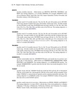
Figure 32.35 shows the orthogonalized responses of
y1
and
y2
to a forecast error impulse in
y1
with
two standard errors.
Figure 32.35 Plot of Orthogonalized Impulse Response
Forecasting
The optimal (minimum MSE) l-step-ahead forecast of y
tCl
is
y
tCljt
D
p
X
j D1
ˆ
j
y
tClj jt
C
s
X
j D0
‚

j

x
tClj jt

q
X
j Dl
‚
j

tClj
; l Ä q
y
tCljt
D
p
X
j D1
ˆ
j
y
tClj jt
C
s
X
j D0
‚

j
x
tClj jt

; l > q
with
y
tClj jt
D y
tClj
and
x
tClj jt
D x
tClj
for
l Ä j
. For the forecasts
x
tClj jt
, see the
section “State-Space Representation” on page 2105.
Forecasting ✦ 2123
Covariance Matrices of Prediction Errors without Exogenous (Independent) Variables
Under the stationarity assumption, the optimal (minimum MSE)
l
-step-ahead forecast of
y
tCl
has
an infinite moving-average form,
y
tCljt
D

P
1
j Dl
‰
j

tClj
. The prediction error of the optimal
l
-step-ahead forecast is
e
tCljt
D y
tCl
y
tCljt
D
P
l1
j D0
‰
j

tClj
, with zero mean and covariance
matrix,
†.l/ D Cov.e
tCljt
/ D
l1

X
j D0
‰
j
†‰
0
j
D
l1
X
j D0
‰
o
j
‰
o
0
j
where
‰
o
j
D ‰
j
P
with a lower triangular matrix
P
such that
† D PP
0

. Under the assumption of
normality of the

t
, the
l
-step-ahead prediction error
e
tCljt
is also normally distributed as multivariate
N.0; †.l//
. Hence, it follows that the diagonal elements

2
i i
.l/
of
†.l/
can be used, together with
the point forecasts
y
i;tCljt
, to construct
l
-step-ahead prediction intervals of the future values of the
component series, y
i;tCl
.
The following statements use the COVPE option to compute the covariance matrices of the prediction
errors for a VAR(1) model. The parts of the VARMAX procedure output are shown in Figure 32.36

and Figure 32.37.
proc varmax data=simul1;
model y1 y2 / p=1 noint lagmax=5
printform=both
print=(decompose(5) impulse=(all) covpe(5));
run;
Figure 32.36 is the output in a matrix format associated with the COVPE option for the prediction
error covariance matrices.
Figure 32.36 Covariances of Prediction Errors (COVPE Option)
The VARMAX Procedure
Prediction Error Covariances
Lead Variable y1 y2
1 y1 1.28875 0.39751
y2 0.39751 1.41839
2 y1 2.92119 1.00189
y2 1.00189 2.18051
3 y1 4.59984 1.98771
y2 1.98771 3.03498
4 y1 5.91299 3.04856
y2 3.04856 4.07738
5 y1 6.69463 3.85346
y2 3.85346 5.07010
Figure 32.37 is the output in a univariate format associated with the COVPE option for the prediction
error covariances. This printing format more easily explains the prediction error covariances of each
variable.
2124 ✦ Chapter 32: The VARMAX Procedure
Figure 32.37 Covariances of Prediction Errors
Prediction Error Covariances by Variable
Variable Lead y1 y2
y1 1 1.28875 0.39751

2 2.92119 1.00189
3 4.59984 1.98771
4 5.91299 3.04856
5 6.69463 3.85346
y2 1 0.39751 1.41839
2 1.00189 2.18051
3 1.98771 3.03498
4 3.04856 4.07738
5 3.85346 5.07010
Covariance Matrices of Prediction Errors in the Presence of Exogenous (Independent)
Variables
Exogenous variables can be both stochastic and nonstochastic (deterministic) variables. Considering
the forecasts in the VARMAX(p,q,s) model, there are two cases.
When exogenous (independent) variables are stochastic (future values not specified):
As defined in the section “State-Space Representation” on page 2105, y
tCljt
has the representation
y
tCljt
D
1
X
j Dl
V
j
a
tClj
C
1
X

j Dl
‰
j

tClj
and hence
e
tCljt
D
l1
X
j D0
V
j
a
tClj
C
l1
X
j D0
‰
j

tClj
Therefore, the covariance matrix of the l-step-ahead prediction error is given as
†.l/ D Cov.e
tCljt
/ D
l1
X

j D0
V
j
†
a
V
0
j
C
l1
X
j D0
‰
j
†

‰
0
j
where
†
a
is the covariance of the white noise series
a
t
, and
a
t
is the white noise series for the
VARMA(

p
,
q
) model of exogenous (independent) variables, which is assumed not to be correlated
with 
t
or its lags.
Forecasting ✦ 2125
When future exogenous (independent) variables are specified:
The optimal forecast
y
tCljt
of
y
t
conditioned on the past information and also on known future
values x
tC1
; : : : ; x
tCl
can be represented as
y
tCljt
D
1
X
j D0
‰

j

x
tClj
C
1
X
j Dl
‰
j

tClj
and the forecast error is
e
tCljt
D
l1
X
j D0
‰
j

tClj
Thus, the covariance matrix of the l-step-ahead prediction error is given as
†.l/ D Cov.e
tCljt
/ D
l1
X
j D0
‰
j

†

‰
0
j
Decomposition of Prediction Error Covariances
In the relation
†.l/ D
P
l1
j D0
‰
o
j
‰
o
0
j
, the diagonal elements can be interpreted as providing a
decomposition of the
l
-step-ahead prediction error covariance

2
i i
.l/
for each component series
y
it
into contributions from the components of the standardized innovations 

t
.
If you denote the (i; n)th element of ‰
o
j
by
j;i n
, the MSE of y
i;tChjt
is
MSE.y
i;tChjt
/ D E.y
i;tCh
 y
i;tChjt
/
2
D
l1
X
j D0
k
X
nD1

2
j;i n
Note that
P

l1
j D0

2
j;i n
is interpreted as the contribution of innovations in variable
n
to the prediction
error covariance of the l-step-ahead forecast of variable i.
The proportion,
!
l;in
, of the
l
-step-ahead forecast error covariance of variable
i
accounting for the
innovations in variable n is
!
l;in
D
l1
X
j D0

2
j;i n
=MSE.y
i;tChjt
/

The following statements use the DECOMPOSE option to compute the decomposition of prediction
error covariances and their proportions for a VAR(1) model:
proc varmax data=simul1;
model y1 y2 / p=1 noint print=(decompose(15))
printform=univariate;
run;
2126 ✦ Chapter 32: The VARMAX Procedure
The proportions of decomposition of prediction error covariances of two variables are given in
Figure 32.38. The output explains that about 91.356% of the one-step-ahead prediction error
covariances of the variable
y
2t
is accounted for by its own innovations and about 8.644% is accounted
for by y
1t
innovations.
Figure 32.38 Decomposition of Prediction Error Covariances (DECOMPOSE Option)
Proportions of Prediction Error
Covariances by Variable
Variable Lead y1 y2
y1 1 1.00000 0.00000
2 0.88436 0.11564
3 0.75132 0.24868
4 0.64897 0.35103
5 0.58460 0.41540
y2 1 0.08644 0.91356
2 0.31767 0.68233
3 0.50247 0.49753
4 0.55607 0.44393
5 0.53549 0.46451

Forecasting of the Centered Series
If the CENTER option is specified, the sample mean vector is added to the forecast.
Forecasting of the Differenced Series
If dependent (endogenous) variables are differenced, the final forecasts and their prediction error
covariances are produced by integrating those of the differenced series. However, if the PRIOR
option is specified, the forecasts and their prediction error variances of the differenced series are
produced.
Let
z
t
be the original series with some appended zero values that correspond to the unobserved past
observations. Let
.B/
be the
k  k
matrix polynomial in the backshift operator that corresponds to
the differencing specified by the MODEL statement. The off-diagonal elements of

i
are zero, and
the diagonal elements can be different. Then y
t
D .B/z
t
.
This gives the relationship
z
t
D 
1

.B/y
t
D
1
X
j D0
ƒ
j
y
tj
where 
1
.B/ D
P
1
j D0
ƒ
j
B
j
and ƒ
0
D I
k
.
The l-step-ahead prediction of z
tCl
is
z
tCljt

D
l1
X
j D0
ƒ
j
y
tClj jt
C
1
X
j Dl
ƒ
j
y
tClj
Tentative Order Selection ✦ 2127
The l-step-ahead prediction error of z
tCl
is
l1
X
j D0
ƒ
j

y
tClj
 y
tClj jt


D
l1
X
j D0
0
@
j
X
uD0
ƒ
u
‰
j u
1
A

tClj
Letting †
z
.0/ D 0, the covariance matrix of the l-step-ahead prediction error of z
tCl
, †
z
.l/, is
†
z
.l/ D
l1
X

j D0
0
@
j
X
uD0
ƒ
u
‰
j u
1
A
†

0
@
j
X
uD0
ƒ
u
‰
j u
1
A
0
D †
z
.l  1/ C
0

@
l1
X
j D0
ƒ
j
‰
l1j
1
A
†

0
@
l1
X
j D0
ƒ
j
‰
l1j
1
A
0
If there are stochastic exogenous (independent) variables, the covariance matrix of the l-step-ahead
prediction error of z
tCl
, †
z
.l/, is

†
z
.l/ D †
z
.l  1/ C
0
@
l1
X
j D0
ƒ
j
‰
l1j
1
A
†

0
@
l1
X
j D0
ƒ
j
‰
l1j
1
A
0

C
0
@
l1
X
j D0
ƒ
j
V
l1j
1
A
†
a
0
@
l1
X
j D0
ƒ
j
V
l1j
1
A
0
Tentative Order Selection
Sample Cross-Covariance and Cross-Correlation Matrices
Given a stationary multivariate time series y
t

, cross-covariance matrices are
.l/ D EŒ.y
t
 /.y
tCl
 /
0

where  D E.y
t
/, and cross-correlation matrices are
.l/ D D
1
.l/D
1
where D is a diagonal matrix with the standard deviations of the components of y
t
on the diagonal.
The sample cross-covariance matrix at lag l, denoted as C.l/, is computed as
O
.l/ D C.l/ D
1
T
T l
X
tD1
Q
y
t
Q

y
0
tCl
2128 ✦ Chapter 32: The VARMAX Procedure
where
Q
y
t
is the centered data and
T
is the number of nonmissing observations. Thus,
O
.l/
has
.i; j /th element O
ij
.l/ D c
ij
.l/. The sample cross-correlation matrix at lag l is computed as
O
ij
.l/ D c
ij
.l/=Œc
i i
.0/c
jj
.0/
1=2
; i; j D 1; : : : ; k

The following statements use the CORRY option to compute the sample cross-correlation matrices
and their summary indicator plots in terms of
C; ;
and

, where
C
indicates significant positive
cross-correlations,

indicates significant negative cross-correlations, and

indicates insignificant
cross-correlations.
proc varmax data=simul1;
model y1 y2 / p=1 noint lagmax=3 print=(corry)
printform=univariate;
run;
Figure 32.39 shows the sample cross-correlation matrices of
y
1t
and
y
2t
. As shown, the sample
autocorrelation functions for each variable decay quickly, but are significant with respect to two
standard errors.
Figure 32.39 Cross-Correlations (CORRY Option)
The VARMAX Procedure
Cross Correlations of Dependent Series by Variable

Variable Lag y1 y2
y1 0 1.00000 0.67041
1 0.83143 0.84330
2 0.56094 0.81972
3 0.26629 0.66154
y2 0 0.67041 1.00000
1 0.29707 0.77132
2 -0.00936 0.48658
3 -0.22058 0.22014
Schematic Representation
of Cross Correlations
Variable/
Lag 0 1 2 3
y1 ++ ++ ++ ++
y2 ++ ++ .+ -+
+ is > 2
*
std error, - is <
-2
*
std error, . is between
Tentative Order Selection ✦ 2129
Partial Autoregressive Matrices
For each
m D 1; 2; : : : ; p
you can define a sequence of matrices
ˆ
mm
, which is called the partial
autoregression matrices of lag

m
, as the solution for
ˆ
mm
to the Yule-Walker equations of order
m
,
.l/ D
m
X
iD1
.l i /ˆ
0
im
; l D 1; 2; : : : ; m
The sequence of the partial autoregression matrices
ˆ
mm
of order
m
has the characteristic property
that if the process follows the AR(
p
), then
ˆ
pp
D ˆ
p
and
ˆ

mm
D 0
for
m > p
. Hence, the
matrices
ˆ
mm
have the cutoff property for a VAR(
p
) model, and so they can be useful in the
identification of the order of a pure VAR model.
The following statements use the PARCOEF option to compute the partial autoregression matrices:
proc varmax data=simul1;
model y1 y2 / p=1 noint lagmax=3
printform=univariate
print=(corry parcoef pcorr
pcancorr roots);
run;
Figure 32.40 shows that the model can be obtained by an AR order
m D 1
since partial autoregression
matrices are insignificant after lag 1 with respect to two standard errors. The matrix for lag 1 is the
same as the Yule-Walker autoregressive matrix.
Figure 32.40 Partial Autoregression Matrices (PARCOEF Option)
The VARMAX Procedure
Partial Autoregression
Lag Variable y1 y2
1 y1 1.14844 -0.50954
y2 0.54985 0.37409

2 y1 -0.00724 0.05138
y2 0.02409 0.05909
3 y1 -0.02578 0.03885
y2 -0.03720 0.10149
Schematic Representation
of Partial Autoregression
Variable/
Lag 1 2 3
y1 +-
y2 ++
+ is > 2
*
std error, - is <
-2
*
std error, . is between
2130 ✦ Chapter 32: The VARMAX Procedure
Partial Correlation Matrices
Define the forward autoregression
y
t
D
m1
X
iD1
ˆ
i;m1
y
ti
C u

m;t
and the backward autoregression
y
tm
D
m1
X
iD1
ˆ

i;m1
y
tmCi
C u

m;t m
The matrices P .m/ defined by Ansley and Newbold (1979) are given by
P .m/ D †
1=2
m1
ˆ
0
mm
†
1=2
m1
where
†
m1
D Cov.u

m;t
/ D .0/ 
m1
X
iD1
.i /ˆ
0
i;m1
and
†

m1
D Cov.u

m;t m
/ D .0/ 
m1
X
iD1
.m  i/ˆ

0
mi;m1
P .m/
are the partial cross-correlation matrices at lag
m
between the elements of
y
t
and

y
tm
, given
y
t1
; : : : ; y
tmC1
. The matrices
P .m/
have the cutoff property for a VAR(
p
) model, and so they
can be useful in the identification of the order of a pure VAR structure.
The following statements use the PCORR option to compute the partial cross-correlation matrices:
proc varmax data=simul1;
model y1 y2 / p=1 noint lagmax=3
print=(pcorr)
printform=univariate;
run;
The partial cross-correlation matrices in Figure 32.41 are insignificant after lag 1 with respect to two
standard errors. This indicates that an AR order of m D 1 can be an appropriate choice.
Tentative Order Selection ✦ 2131
Figure 32.41 Partial Correlations (PCORR Option)
The VARMAX Procedure
Partial Cross Correlations by Variable
Variable Lag y1 y2
y1 1 0.80348 0.42672
2 0.00276 0.03978
3 -0.01091 0.00032
y2 1 -0.30946 0.71906

2 0.04676 0.07045
3 0.01993 0.10676
Schematic Representation of
Partial Cross Correlations
Variable/
Lag 1 2 3
y1 ++
y2 -+
+ is > 2
*
std error, - is <
-2
*
std error, . is between
Partial Canonical Correlation Matrices
The partial canonical correlations at lag
m
between the vectors
y
t
and
y
tm
, given
y
t1
; : : : ; y
tmC1
,
are

1  
1
.m/  
2
.m/   
k
.m/
. The partial canonical correlations are the canonical cor-
relations between the residual series
u
m;t
and
u

m;t m
, where
u
m;t
and
u

m;t m
are defined in the
previous section. Thus, the squared partial canonical correlations

2
i
.m/
are the eigenvalues of the
matrix

fCov.u
m;t
/g
1
E.u
m;t
u

0
m;t m
/fCov.u

m;t m
/g
1
E.u

m;t m
u
0
m;t
/ D ˆ

0
mm
ˆ
0
mm
It follows that the test statistic to test for
ˆ

m
D 0
in the VAR model of order
m > p
is approximately
.T  m/ tr fˆ

0
mm
ˆ
0
mm
g  .T  m/
k
X
iD1

2
i
.m/
and has an asymptotic chi-square distribution with k
2
degrees of freedom for m > p.
The following statements use the PCANCORR option to compute the partial canonical correlations:
proc varmax data=simul1;
model y1 y2 / p=1 noint lagmax=3 print=(pcancorr);
run;