SAS/ETS 9.22 User''''s Guide 269 pptx

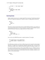
2672 ✦ Chapter 40: Creating Time ID Variables
Figure 40.5 Create Time ID Variable Window
Select the
OK
button. This opens the
New Data Set Name
window. Enter “OBS_ID” in the
New
data set name field. Enter “T” in the New ID variable name field.
Now select the
OK
button. The new data set OBS_ID is created, and the system returns to the
Data
Set Selection window, which now appears as shown in Figure 40.6.
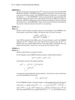
Using Observation Numbers as the Time ID ✦ 2673
Figure 40.6 Data Set Selection Window after Creating Time ID
The
Interval
field for OBS_ID has the value ‘1’. This means that the values of the time ID variable
T increment by one between successive observations.
Select the Table button to look at the OBS_ID data set, as shown in Figure 40.7.
2674 ✦ Chapter 40: Creating Time ID Variables
Figure 40.7 VIEWTABLE of Data Set with Observation Index ID
Select
File
and
Close
to close the VIEWTABLE window. Select the
OK
button from the
Data Set

Selection window to return to the Time Series Forecasting window.
Creating a Time ID from Other Dating Variables
Your data set might contain ID variables that date the observations in a different way than the SAS
date valued ID variable expected by the forecasting system. For example, for monthly data, the data
set might contain the ID variables YEAR and MONTH, which together date the observations.
In these cases, you can use the Forecasting System’s Create Time ID features to compute a time ID
variable with SAS date values from the existing dating variables. As an example of this, use the SAS
data set read in by the following SAS statements:
Creating a Time ID from Other Dating Variables ✦ 2675
data id_parts;
input yr qtr y;
datalines;
91 1 10
91 2 15
91 3 20
91 4 25
92 1 30
92 2 35
92 3 40
92 4 45
93 1 50
93 2 55
93 3 60
93 4 65
94 1 70
94 2 75
94 3 80
94 4 85
run;
Submit these SAS statements to create the data set ID_PARTS. This data set contains the three

variables YR, QTR, and Y. YR and QTR are ID variables that together date the observations, but
each variable provides only part of the date information. Because the forecasting system requires a
single dating variable containing SAS date values, you need to combine YR and QTR to create a
single variable DATE.
Type “ID_PARTS” in the
Data Set
field and press the ENTER key. (You could also use the Browse
button to open the Data Set Selection window, as in the previous example, and complete this example
from there.)
Select the Create button at the right of the
Time ID
field. This opens the menu of Create Time ID
choices, as shown in Figure 40.8.
2676 ✦ Chapter 40: Creating Time ID Variables
Figure 40.8 Adding a Time ID Variable
Select the second choice,
Create from existing variables
. This opens the window shown in
Figure 40.9.
Creating a Time ID from Other Dating Variables ✦ 2677
Figure 40.9 Creating a Time ID Variable from Date Parts
In the Variables list, select YR. In the Date Part list, select YEAR as shown in Figure 40.10.
2678 ✦ Chapter 40: Creating Time ID Variables
Figure 40.10 Specifying the ID Variable for Years
Now click the right-pointing arrow button. The variable YR and the part code YEAR are added to
the Existing Time IDs list.
Next select QTR from the
Variables
list, select QTR from the
Date Part

list, and click the arrow
button. This adds the variable QTR and the part code QTR to the
Existing Time IDs
list, as
shown in Figure 40.11.
Creating a Time ID from Other Dating Variables ✦ 2679
Figure 40.11 Creating a Time ID Variable from Date Parts
Now select the
OK
button. This opens the
New Data Set Name
window. Change the
New data
set name field to NEWDATE, and then select the OK button.
The data set NEWDATE is created, and the system returns to the
Time Series Forecasting
window with NEWDATE as the selected Data Set. The Time ID field is set to DATE, and the Interval
field is set to QTR.
2680
Chapter 41
Specifying Forecasting Models
Contents
Series Diagnostics . . . . . . . . . . . . . . . . . . . . . . . . . . . . . . . . . . . 2681
Models to Fit Window . . . . . . . . . . . . . . . . . . . . . . . . . . . . . . . . 2685
Automatic Model Selection . . . . . . . . . . . . . . . . . . . . . . . . . . . . . . . 2687
Smoothing Model Specification Window . . . . . . . . . . . . . . . . . . . . . . . 2690
ARIMA Model Specification Window . . . . . . . . . . . . . . . . . . . . . . . . 2693
Factored ARIMA Model Specification Window . . . . . . . . . . . . . . . . . . . 2696
Custom Model Specification Window . . . . . . . . . . . . . . . . . . . . . . . . 2700
Editing the Model Selection List . . . . . . . . . . . . . . . . . . . . . . . . . . . 2706

Forecast Combination Model Specification Window . . . . . . . . . . . . . . . . . 2710
Incorporating Forecasts from Other Sources . . . . . . . . . . . . . . . . . . . . . 2713
This chapter explores the tools available through the Develop Models window for investigating
the properties of time series and for specifying and fitting models. The first section shows you
how to diagnose time series properties in order to determine the class of models appropriate for
forecasting series with such properties. Later sections show you how to specify and fit different kinds
of forecasting models.
Series Diagnostics
The series diagnostics tool helps you determine the kinds of forecasting models that are appropriate
for the data series so that you can limit the search for the best forecasting model. The series
diagnostics address these three questions: Is a log transformation needed to stabilize the variance? Is
a time trend present in the data? Is there a seasonal pattern to the data?
The automatic model fitting process, which you used in the previous chapter through the Automatic
Model Fitting window, performs series diagnostics and selects trial models from a list according to
the results. You can also look at the diagnostic information and make your own decisions as to the
kinds of models appropriate for the series. The following example illustrates the series diagnostics
features.
Select “Develop Models” from the Time Series Forecasting window. Select the library SASHELP, the
data set CITIMON, and the series RCARD. This series represents domestic retail sales of passenger
cars. To look at this series, select “View Series” from the Develop Models window. This opens the
Time Series Viewer window, as shown in Figure 41.1.