SAS/ETS 9.22 User''''s Guide 276 docx

2742 ✦ Chapter 43: Using Predictor Variables
Linear Trend
From the Develop Models window, select
Fit ARIMA Model.
From the ARIMA Model Specifica-
tion window, select Add and then select Linear Trend from the menu (shown in Figure 43.1).
A linear trend is added to the Predictors list, as shown in Figure 43.3.
Figure 43.3 Linear Trend Predictor Specified
The description for the linear trend item shown in the Predictors list has the following meaning.
The first part of the description, Trend Curve, describes the type of predictor. The second part,
_LINEAR_, gives the variable name of the predictor series. In this case, the variable is a time index
that the system computes. This variable is included in the output forecast data set. The final part,
Linear Trend, describes the predictor.
Notice that the model you have specified consists only of the time index regressor _LINEAR_ and an
intercept. Although this window is normally used to specify ARIMA models, in this case no ARIMA
model options are specified, and the model is a simple regression on time.
Select the
OK
button. The Linear Trend model is fit and added to the model list in the Develop Models
window.
Time Trend Curves ✦ 2743
Now open the Model Viewer by using the
View Model Graphically
icon or the
Model
Predictions
item under the
View
pull-down menu or toolbar. This displays a plot of the model
predictions and actual series values, as shown in Figure 43.4. The predicted values lie along the least
squares trend line.

Figure 43.4 Linear Trend Model
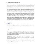
Time Trend Curves
From the Develop Models window, select
Fit ARIMA Model
. From the ARIMA Model Specifica-
tion window, select
Add
and then select
Trend Curve
from the menu (shown in Figure 43.1). A
menu of different kinds of trend curves is displayed, as shown in Figure 43.5.
2744 ✦ Chapter 43: Using Predictor Variables
Figure 43.5 Time Trend Curves Menu
These trend curves work in a similar way as the Linear Trend option (which is a special case of a
trend curve and one of the choices on the menu), but with the Trend Curve menu you have a choice
of various nonlinear time trends.
Select
Quadratic Trend
. This adds a quadratic time trend to the Predictors list, as shown in
Figure 43.6.
Time Trend Curves ✦ 2745
Figure 43.6 Quadratic Trend Specified
Now select the
OK
button. The quadratic trend model is fit and added to the list of models in the
Develop Models window. The Model Viewer displays a plot of the quadratic trend model, as shown
in Figure 43.7.
2746 ✦ Chapter 43: Using Predictor Variables
Figure 43.7 Quadratic Trend Model
This curve does not fit the PETROL series very well, but the View Model plot illustrates how time

trend models work. You might want to experiment with different trend models to see what the
different trend curves look like.
Some of the trend curves require transforming the dependent series. When you specify one of these
curves, a notice is displayed reminding you that a transformation is needed, and the Transformation
field is automatically filled in. Therefore, you cannot control the Transformation specification when
some kinds of trend curves are specified.
See the section “Time Trend Curves” on page 2743 in Chapter 46, “Forecasting Process Details,” for
more information about the different trend curves.
Regressors ✦ 2747
Regressors
From the Develop Models window, select
Fit ARIMA Model.
From the ARIMA Model Specifica-
tion window, select
Add
and then select
Regressors
from the menu (shown in Figure 43.1). This
displays the
Regressors Selection
window, as shown in Figure 43.8. This window allows you
to select any number of other series in the input data set as regressors to predict the dependent series.
Figure 43.8 Regressors Selection Window
For this example, select
CHEMICAL, Sales: Chemicals and Allied Products
, and
VEHICLES, Sales: Motor Vehicles and Parts
. (Note: You do not need to use the CTRL
key when selecting more than one regressor.) Then select the
OK

button. The two variables you
selected are added to the Predictors list as regressor type predictors, as shown in Figure 43.9.
2748 ✦ Chapter 43: Using Predictor Variables
Figure 43.9 Regressors Selected
You must have forecasts of the future values of the regressor variables in order to use them as
predictors. To do this, you can specify a forecasting model for each regressor, have the system
automatically select forecasting models for the regressors, or supply predicted future values for the
regressors in the input data set.
Even if you have supplied future values for a regressor variable, the system requires a forecasting
model for the regressor. Future values that you supply in the input data set take precedence over
predicted values from the regressor’s forecasting model when the system computes the forecasts for
the dependent series.
Select the
OK
button. The system starts to fit the regression model but then stops and displays a
warning that the regressors that you selected do not have forecasting models, as shown in Figure 43.10.
Regressors ✦ 2749
Figure 43.10 Regressors Needing Models Warning
If you want the system to create forecasting models automatically for the regressor variables by using
the automatic model selection process, select the
OK
button. If not, you can select the
Cancel
button
to abort fitting the regression model.
For this example, select the
OK
button. The system now performs the automatic model selection
process for CHEMICAL and VEHICLES. The selected forecasting models for CHEMICAL and
VEHICLES are added to the model lists for those series. If you switch the current time series in the

Develop Models window to CHEMICAL or VEHICLES, you will see the model that the system
selected for that series.
Once forecasting models have been fit for all regressors, the system proceeds to fit the regression
model for PETROL. The fitted regression model is added to the model list displayed in the Develop
Models window.
2750 ✦ Chapter 43: Using Predictor Variables
Adjustments
An adjustment predictor is a variable in the input data set that is used to adjust the forecast values
produced by the forecasting model. Unlike a regressor, an adjustment variable does not have a
regression coefficient. No model fitting is performed for adjustments. Nonmissing values of the
adjustment series are simply added to the model prediction for the corresponding period. Missing
adjustment values are ignored. If you supply adjustment values for observations within the period of
fit, the adjustment values are subtracted from the actual values, and the model is fit to these adjusted
values.
To add adjustments, select
Add
and then select
Adjustments
from the pop-up menu (shown in
Figure 43.1). This displays the
Adjustments Selection
window. The Adjustments Selection
window functions the same as the Regressor Selection window (which is shown in Figure 43.8). You
can select any number of adjustment variables as predictors.
Unlike regressors, adjustments do not require forecasting models for the adjustment variables. If a
variable that is used as an adjustment does have a forecasting model fit to it, the adjustment variable’s
forecasting model is ignored when the variable is used as an adjustment.
You can use forecast adjustments to account for expected future events that have no precedent in the
past and so cannot be modeled by regression. For example, suppose you are trying to forecast the
sales of a product, and you know that a special promotional campaign for the product is planned

during part of the period you want to forecast. If such sales promotion programs have been frequent
in the past, then you can record the past and expected future level of promotional efforts in a variable
in the data set and use that variable as a regressor in the forecasting model.
However, if this is the first sales promotion of its kind for this product, you have no way to estimate
the effect of the promotion from past data. In this case, the best you can do is to make an educated
guess at the effect the promotion will have and add that guess to what your forecasting model would
predict in the absence of the special sales campaign.
Adjustments are also useful for making judgmental alterations to forecasts. For example, suppose
you have produced forecast sales data for the next 12 months. Your supervisor believes that the
forecasts are too optimistic near the end and asks you to prepare a forecast graph in which the
numbers that you have forecast are reduced by 1000 in the last three months. You can accomplish
this task by editing the input data set so that it contains observations for the actual data range of
sales plus 12 additional observations for the forecast period, and a new variable called, for example,
ADJUSTMENT. The variable ADJUSTMENT contains the value 1000 for the last three observations
and is missing for all other observations. You fit the same model previously selected for forecasting by
using the
ARIMA Model Specification
or
Custom Model Specification
window, but with
an adjustment added that uses the variable ADJUSTMENT. Now when you graph the forecasts by
using the Model Viewer, the last three periods of the forecast are reduced by 1000. The confidence
limits are unchanged, which helps draw attention to the fact that the adjustments to the forecast
deviate from what would be expected statistically.
Dynamic Regressor ✦ 2751
Dynamic Regressor
Selecting
Dynamic Regressor
from the
Add Predictors

menu (shown in Figure 43.1) allows
you to specify a complex time series model of the way that a predictor variable influences the series
that you are forecasting.
When you specify a predictor variable as a simple regressor, only the current period value of the
predictor effects the forecast for the period. By specifying the predictor with the Dynamic Regression
option, you can use past values of the predictor series, and you can model effects that take place
gradually.
Dynamic regression models are an advanced feature that you are unlikely to find useful unless you
have studied the theory of statistical time series analysis. You might want to skip this section if you
are not trained in time series modeling.
The term dynamic regression was introduced by Pankratz (1991) and refers to what Box and Jenkins
(1976) named transfer function models. In dynamic regression, you have a time series model, similar
to an ARIMA model, that predicts how changes in the predictor series affect the dependent series
over time.
The dynamic regression model relates the predictor variable to the expected value of the dependent
series in the same way that an ARIMA model relates the fluctuations of the dependent series about
its conditional mean to the random error term (which is also called the innovation series). Refer
to Pankratz (1991) and Box and Jenkins (1976) for more information about dynamic regression or
transfer function models. See also Chapter 7, “The ARIMA Procedure.”
From the Develop Models window, select
Fit ARIMA Model.
From the ARIMA Model Specifica-
tion window, select Add and then select Linear Trend from the menu (shown in Figure 43.1).
Now select
Add
and select
Dynamic Regressor
. This displays the
Dynamic Regressors
Selection window, as shown in Figure 43.11.