SAS/ETS 9.22 User''''s Guide 278 ppsx

2762 ✦ Chapter 43: Using Predictor Variables
The pattern of the series from August 1990 through January 1991 is more complex than a simple
shift in level or trend. For this pattern, you need a complex intervention model for an event that
causes a sharp rise followed by a rapid return to the previous trend line. To specify this model, use
the Effect Time Window and Effect Decay Rate options.
The
Effect Time Window
option controls the number of lags of the intervention’s indicator variable
used to model the effect of the intervention on the dependent series. For a simple intervention, the
number of lags is zero, which means that the effect of the intervention is modeled by fitting a single
regression coefficient to the intervention’s indicator variable.
When you set the number of lags greater than zero, regression coefficients are fit to lags of the
indicator variable. This allows you to model interventions whose effects take place gradually, or to
model rebound effects. For example, severe weather might reduce production during one period but
cause an increase in production in the following period as producers struggle to catch up. You could
model this by using a point intervention with an effect time window of 1 lag. This would fit two
coefficients for the intervention, one for the immediate effect and one for the delayed effect.
The
Effect Decay Pattern
option controls how the effect of the intervention dissipates over time.
None
specifies that there is no gradual decay: for point interventions, the effect ends immediately; for
step and ramp interventions, the effect continues indefinitely.
Exp
specifies that the effect declines at
an exponential rate.
Wave
specifies that the effect declines like an exponentially damped sine wave
(or as the sum of two exponentials, depending on the fit to the data).
If you are familiar with time series analysis, these options might be clearer if you note that together
the Effect Time Window and Effect Decay Pattern options define the numerator and denominator

orders of a transfer function or dynamic regression model for the indicator variable of the intervention.
See the section “Dynamic Regressor” on page 2751 for more information.
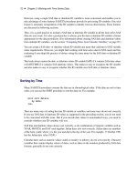
For this example, select 2 lags as the value of the Event Time Window option, and select
Exp
as the
Effect Decay Pattern option. The window should now appear as shown in Figure 43.20.
Fitting the Intervention Model ✦ 2763
Figure 43.20 Complex Intervention Model
Select the OK button to add the intervention to the list.
Fitting the Intervention Model
The Interventions for Series window now contains definitions for four intervention predictors. Select
all four interventions, as shown in Figure 43.21.
2764 ✦ Chapter 43: Using Predictor Variables
Figure 43.21 Interventions for Series Window
Select the
OK
button. This returns you to the ARIMA Model Specification window, which now lists
items in the Predictors list, as shown in Figure 43.22.
Fitting the Intervention Model ✦ 2765
Figure 43.22 Linear Trend with Interventions Specified
Select the
OK
button to fit this model. After the model is fit, bring up the Model Viewer. You will see
a plot of the model predictions, as shown in Figure 43.23.
2766 ✦ Chapter 43: Using Predictor Variables
Figure 43.23 Linear Trend with Interventions Model
You can use the Zoom In feature to take a closer look at how the complex intervention effect fits the
excursion in the series starting in August 1990.
Limitations of Intervention Predictors ✦ 2767
Limitations of Intervention Predictors

Note that the model you have just fit is intended only to illustrate the specification of interventions.
It is not intended as an example of good forecasting practice.
The use of continuing (step and ramp type) interventions as predictors has some limitations that you
should consider. If you model a change in trend with a simple ramp intervention, then the trend in
the data before the date of the intervention has no influence on the forecasts. Likewise, when you use
a step intervention, the average level of the series before the intervention has no influence on the
forecasts.
Only the final trend and level at the end of the series are extrapolated into the forecast period. If a
linear trend is the only pattern of interest, then instead of specifying step or ramp interventions, it
would be simpler to adjust the period of fit so that the model ignores the data before the final trend or
level change.
Step and ramp interventions are valuable when there are other patterns in the data—such as season-
ality, autocorrelated errors, and error variance—that are stable across the changes in level or trend.
Step and ramp interventions enable you to fit seasonal and error autocorrelation patterns to the whole
series while fitting the trend only to the latter part of the series.
Point interventions are a useful tool for dealing with outliers in the data. A point intervention will
fit the series value at the specified date exactly, and it has the effect of removing that point from
the analysis. When you specify an effect time window, a point intervention will exactly fit as many
additional points as the number of lags specified.
Seasonal Dummies
A Seasonal Dummies predictor is a special feature that adds to the model seasonal indicator or
“dummy” variables to serve as regressors for seasonal effects.
From the Develop Models window, select
Fit ARIMA Model.
From the ARIMA Model Specifica-
tion window, select
Add
and then select
Seasonal Dummies
from the menu (shown in Figure 43.1).

A Seasonal Dummies input is added to the Predictors list, as shown in Figure 43.24.
2768 ✦ Chapter 43: Using Predictor Variables
Figure 43.24 Seasonal Dummies Specified
Select the
OK
button. A model consisting of an intercept and 11 seasonal dummy variables is fit and
added to the model list in the Develop Models window. This is effectively a mean model with a
separate mean for each month.
Now return to the Model Viewer, which displays a plot of the model predictions and actual series
values, as shown in Figure 43.25. This is obviously a poor model for this series, but it serves to
illustrate how seasonal dummy variables work.
Seasonal Dummies ✦ 2769
Figure 43.25 Seasonal Dummies Model
Now select the parameter estimates icon, the fifth from the top on the vertical toolbar. This displays
the Parameter Estimates table, as shown in Figure 43.26.
2770 ✦ Chapter 43: Using Predictor Variables
Figure 43.26 Parameter Estimates for Seasonal Dummies Model
Since the data for this example are monthly, the Seasonal Dummies option added 11 seasonal dummy
variables. These include a dummy regressor variable that is 1.0 for January and 0 for other months, a
regressor that is 1.0 only for February, and so forth through November.
Because the model includes an intercept, no dummy variable is added for December. The December
effect is measured by the intercept, while the effect of other seasons is measured by the difference
between the intercept and the estimated regression coefficient for the season’s dummy variable.
The same principle applies for other data frequencies: the “Seasonal Dummy 1” parameter always
refers to the first period in the seasonal cycle; and, when an intercept is present in the model, there is
no seasonal dummy parameter for the last period in the seasonal cycle.
References ✦ 2771
References
Box, G.E.P. and Jenkins, G.M. (1976), Time Series Analysis: Forecasting and Control, San Francisco:
Holden-Day.

Pankratz, Alan (1991), Forecasting with Dynamic Regression Models, New York: John Wiley &
Sons.