Integrated Research in GRID Computing- P11 potx
Bạn đang xem bản rút gọn của tài liệu. Xem và tải ngay bản đầy đủ của tài liệu tại đây (1.23 MB, 20 trang )
Scheduling
Workflows
with Budget Constraints 191
in defining execution costs of the tasks of the DAG. However, as indicated by
studies on workflow scheduling [2, 7, 12], it appears that heuristics performing
best in a static environment (e.g., HBMCT [8]) have the highest potential to
perform best in a more accurately modelled Grid environment.
In order to solve the problem of scheduling optimally under a budget con-
straint, we propose two basic families of heuristics, which are evaluated in the
paper. The idea in both approaches is to start from an assignment which has
good performance under one of the two optimization criteria considered (that
is,
makespan and budget) and swap tasks between machines trying to optimize
as much as possible for the other criterion. The first approach starts with an
assignment of tasks onto machines that is optimized for makespan (using a
standard algorithm for DAG scheduling onto heterogeneous resources, such as
HEFT [10] or HBMCT [8]). As long as the budget is exceeded, the idea is
to keep swapping tasks between machines by choosing first those tasks where
the largest savings in terms of money will result in the smallest loss in terms
of schedule length. We call this approach as LOSS. Conversely, the second
approach starts with the cheapest assignment of tasks onto resources (that is,
the one that requires the least money). As long as there is budget available, the
idea is to keep swapping tasks between machines by choosing first those tasks
where the largest benefits in terms of minimizing the makespan will be obtained
for the smallest expense. We call this approach GAIN. Variations in how tasks
are chosen result in different heuristics, which we evaluate in the paper.
The rest of the paper is organized as follows. Section 2 gives some back-
ground information about DAGs. In Section 3 we present the core algorithm
proposed along with a description of the two approaches developed and some
variants. In Section 4, we present experimental results that evaluate the two
approaches. Finally, Section 5 concludes the paper.
2.
Background
Following similar studies [2, 12, 9], the DAG model we adopt makes the
following assumptions. Without loss of generality, we consider that a DAG
starts with a single entry node and has a single exit node. Each node connects
to other nodes with edges, which represent the node dependencies. Edges are
annotated with a value, which indicates the amount of data that need to be
communicated from a parent node to a child node. For each node the execution
time on each different machine available is given. In addition, the time to
communicate data between machines is given. Using this input, traditional
studies from the literature aim to assign tasks onto machines in such a way that
the overall schedule length is minimized and precedence constraints are met.
An example of a DAG and the schedule length produced using a well-known
heuristic, HEFT [10], is shown in Figure 1. A number of other heuristics could
192
INTEGRATED RESEARCH IN GRID COMPUTING
task
0
1
2
3
4
5
6
7
mO
17
26
30
6
12
7
23
12
ml
28
11
13
25
2
8
16
14
m2
17
14
27
3
12
23
29
11
(b) the computation cost of nodes
on three different machines
(a) an example graph
MO Ml M2
machines
mO-
ml
ml - m2
m0-m2
time for a data unit
1.607
0.9
3.0
(c) communication cost between the
machines
node
0
1 1
1
2
3
4
5
6
7
start time
0
17
33.07
43
46.07
48.07
64.14
87.14
finish
time
17
43
46.07
49
48.07
56.07
87.14
99.14
(e) the start time and finish time of
each node in (d)
(d) the schedule derived using the
HEFT algorithm
Figure J. An Example of HEFT scheduling in a DAG workflow.
be used too (see [8], for example). It is noted that in the example in the figure
no task is ever assigned to machine M2. This is primarily due to the high
Scheduling
Workflows
with Budget Constraints 193
communication; since HEFT assigns tasks onto the machine that provides the
earliest finish time, no task ever satisfies this condition.
The contribution of this paper relates to the extension of the traditional DAG
model with one extra condition: the usage of each machine available costs
some money. As a result, an additional constraint needs to be satisfied when
scheduling the DAG, namely, that the overall financial cost of the schedule does
not exceed a certain budget. We define the overall (total) cost as the sum of the
costs of executing each task in the DAG onto a machine, that is,
TotalCost =
J2^iJ^
(^)
where Cij is the cost of executing task i onto machine j and is calculated as
the product of the execution time required by the task on the machine that has
been assigned to, times the cost of this machine, that is,
Cij = MachineCostj x ExecutionTimeij
^
(2)
where MachineCostj, is the cost (in money units) per unit of time to run
something on machine j and ExecutionTimeij is the time task i takes to
execute on machine j. Throughout this paper, we assume that the value of
MachineCostj, for all machines, is given.
3.
The Algorithm
3.1 OutUne
The key idea of the algorithm proposed is to satisfy the budget constraint by
finding the best affordable assignment possible. We define the "best assign-
ment" as the assignment whose execution time is the minimum possible. We
define ^'affordable assignment" as the assignment whose cost does not exceed
the budget available. We also assume that, on the basis of the input given, the
budget available is higher than the cost of the cheapest assignment (that is, the
assignment where tasks are allocated onto the machine where it costs the least
to execute them); this guarantees that there is at least one solution within the
budget available. We also assume that the budget available is less than the cost
of the schedule that can be obtained using a DAG scheduling algorithm that
aims to minimize the makespan, such as HEFT or HBMCT. Without the latter
assumption, there would be no need for further investigation: since the cost
of the schedule produced by the DAG scheduling would be within the budget
available, it would be reasonable to use this schedule.
The algorithm starts with an initial assignment of the tasks onto machines
(schedule) and computes for each reassignment of each task to a different ma-
chine, a weight value associated with that particular change. Those weight
values are tabulated; thus, a weight table is created for each task in the DAG
194
INTEGRATED RESEARCH IN GRID COMPUTING
and each machine. Two alternative approaches for computing the weight val-
ues are proposed, depending on the two choices used for the initial assignment:
either optimal for makespan (approach called LOSS — in this case, the initial
assignment would be produced by an efficient DAG scheduling heuristic [10,
8]),
or cheapest (approach called GAIN — in this case, the initial assignment
would be produced by allocating tasks to the machines where it costs the least
in terms of
money;
we call this as the cheapest assignment); the two approaches
are described in more detail below. Using the weight table, tasks are repeatedly
considered for possible reassignment to a machine, as long as the cost of the
current schedule exceeds the budget (in the case that LOSS is followed), or, until
all possible reassignments would exceed the budget (in the case of GAIN). In
either case, the algorithm will try to reassign any given pair of tasks only once,
so when no reassignment is possible the algorithm will terminate. We illustrate
the key steps of the algorithm in Figure 2.
3.2 The
LOSS
Approach
The LOSS approach uses as an initial assignment the output assignment of
either HEFT [10] orHBMCT[8] DAG scheduling algorithms. If
the
available
budget is bigger or equal to the money cost required for this assignment then
this assignment can be used straightaway and no further action is needed. In
all the other cases that the budget is less than the cost required for the initial
assignment, the
LOSS
approach is invoked. The aim of
this
approach is to make
a change in the schedule (assignment) obtained through HEFT or HBMCT, so
that it will result in the minimum loss in execution time for the largest money
savings. This means that the new schedule has an execution time close to the
time the original assignment would require but with less cost. In order to come
up with such a re-assignment, the LOSS weight values for each task to each
machine are computed as follows:
LossWeight(i, m) = ^'"^_ ^"^^ (3)
where Toid is the time to execute task i on the machine assigned by HEFT
or HBMCT, Tnew is the time to execute Task i on machine m. Also,
Coid
is
the cost of executing task i on the machine given by the HEFT or HBMCT
assignment and
Cnew
is the cost of executing task i on machine m. If
Coid
is
less than or equal to
Cnew
the value of LossWeight is considered zero. The
algorithm keeps trying re-assignments by considering the smallest values of the
LossW eight for all tasks and machines (step 4 of the algorithm in Figure 2).
Scheduling Workflows with Budget Constraints
195
Input:
A
DAG (workflow)
G
with task execution time
and
communication
A
set of
machines with cost
of
executing jobs
A DAG scheduhng algorithm
H
Available Budget
B
Algorithm: (two options: LOSS
and
GAIN)
1) If LOSS
then generate schedule
S
using algorithm
H
else generate schedule
S by
mapping each task onto
the
cheapest machine
2) Build
an
array A[number_of_tasks][number_of-machines]
3)
for
each Task
in G
for each Machine
if,
according
to
Schedule
S,
Task
is
assigned
to
Machine
then A [Task] [Machine]
^ 0
else Compute
the
Weight
for
A [Task] [Machine]
endfor
endfor
4) if LOSS
then condition
^—
(Cost
of
schedule
S > B)
else condition
<—
(Cost
of
schedule
S < B)
While (condition
and not all
possible reassignments have been tried)
if
LOSS
then find
the
smallest non-zero value from A, A[i][j]
else find
the
biggest non-zero value from A, A[i][j]
Re-assign Task
i to
Machine
j in S and
calculate new cost
of S.
if (GAIN
and
cost
of
S
> B)
then invalidate previous reassignment
of
Task
i to
Machine
j.
endwhile
5)
if
(cost
of
schedule
S > B)
then
use
cheapest assignment
for S.
6) Return
S
Figure 2.
The
Basic Steps
of
the Proposed Algorithm
3.3
The
GAIN Approach
The
GAIN
approach uses as a starting assignment the assignment that requires
the least money. Each task
is
initially assigned
to the
machine that executes
the task with
the
smallest cost. This assignment
is
called
the
Cheapest Assign-
ment.
In
this variation
of the
algorithm,
the
idea
is to
change
the
Cheapest
Assignment
by
keeping re-assigning tasks
to the
machine where there
is go-
ing
to be the
biggest benefit
in
makespan
for the
smallest money cost. This
is
repeated until there
is no
more money available (budget exceeded).
In a way
similar
to
Equation
3,
weight values
are
computed
as
follows.
It is
noted that
tasks
are
considered
for
reassignment starting with those that have
the
largest
196
INTEGRATED RESEARCH IN GRID COMPUTING
GainWeight value.
GainWeight{i^m) = -^ ^^^^ (4)
where TOM, Tnew,
Cnew^
Cold
have exactly the same meaning as in the LOSS
approach. Furthermore, if
Tnew
is greater than
Toid
or
Cnew
is equal to
Coid
we assign a weight value of zero.
3.4 Variants
For each of the two approaches above, we consider three different variants
which relate to the way that the weights in Equations 3 and 4 are computed;
these modifications result in slightly different versions of the heuristics. The
three variants are:
• LOSSl and GAINI: in this case, the weights are computed exactly as
described above.
• L0SS2 and GAIN2: in this case, the values of
Toid,
Tnew^
and
Cnew^
CQU
in Equations 3 and 4 refer to the benefit in terms of
the
overall makespan
and the overall cost for the schedule and not the benefit associated with
the individual tasks being considered for reassignment.
• L0SS3 and GAIN3: in this case, the weights, computed as shown by
Equations 3 and 4, are recomputed each time a reassignment is made by
the algorithm.
4.
Experimental Results
4.1 Experiment Setup
The algorithm described in the previous section was incorporated in a tool
developed at the University of Manchester, for the evaluation of different DAG
scheduling algorithms
[8-9].
In order to evaluate each version of both ap-
proaches we run the algorithm proposed in this paper with four different types
of DAGs used in the relevant literature
[8-9]:
FFT, Fork-Join (denoted by FRJ),
Laplace (denoted by LPL) and Random
DAGs,
generated as indicated in
[13,
8].
All DAGs contain about 100 nodes each and they are scheduled on 3 different
machines. We run the algorithm proposed in the paper 100 times for each type
of DAG and both approaches and their variants, and we considered the average
values. In each case, we considered nine values for the possible budget, B, as
follows:
B =
Ccheapest
+ k X {CDAG "
Ccheapest)-)
(5)
where Co
AG
is the total cost of the assignment produced by the DAG schedul-
ing heuristic used for the initial assignment (that is, HEFT or HBMCT) when
Scheduling Workflows with Budget Constraints
197
the LOSS approach
is
considered
and
Ccheapest
is the
cost
of the
cheapest
as-
signment. The value
of
A:
varies between 0.1 and 0.9. Essentially, this approach
allows
us to
consider values
of
budget that
lie in ten
equally distanced points
between
the
money cost
for
the cheapest assignment
and
the money cost
for
the
schedule generated
by
HEFT
or
HBMCT. Clearly, values
for
budget outside
those
two
ends
are
trivial
to
handle since they indicate that either there
is no
solution satisfying
the
given budget,
or
HEFT and/or HBMCT
can
provide
a
solution within
the
budget.
4.2 Results
Average Normalized Difference metric:
In
order to compare the quality
of
the schedule produced by the algorithm for each of the six variants and each type
of
DAG,
and
since 100 experiments
are
considered
in
each case,
we
normalize
the schedule length (makespan) using
the
following formula:
-'•value
~
-^cheapest
z^x
Tj^
7^ ) (6)
J-DAG
~
-i-cheapest
where
Tyaiue is the
makespan returned
by
our algorithm,
Tcheapest is the
makespan
of the cheapest assignment and
TJJAG
is the makespan of HEFT or
HBMCT.
As
a general rule,
the
makespan
of
the cheapest assignment,
Tcheapesu
is
expected
to
be the
worst (longest),
and the
makespan
of
HEFT
or
HBMCT,
TDAG, the
best (shortest).
As a
result,
the
formula above
is
expected
to
return
a
value
between
0 and 1
indicating
how
close
the
algorithm
was to
each
of the two
bounds (note that since HEFT
or
HBMCT
are
greedy heuristcs, occasional
values which
are
better than
the
values obtained
by
those
two
heuristics
may
occur).
Hence,
for
comparison purposes, larger values
in
Equation
6
indicate
a
shorter makespan. Since
for
each case
we
take 100 runs,
the
average value
of
the quantity above produces
the
Average Normalized Difference (AND) from
the worst
and the
best, that
is,
.
100 /rpi _rpi \
A
]\T
j-^
^ V"^ (
value cheapest
\ .^^
100^
T^ ^T^ ' ^ ^
^^^
i=l \^DAG
-^cheapest/
where
the
superscript
i
denotes
the i-th run.
Results showing the AND for each different type of DAG, variant, and budget
available (shown
in
terms
of
the value
of
A:
—
see Equation
5) are
presented
in
Figures 3,
4 and
5. Each figure groups the results
of
a
different approach: LOSS
starting with HEFT, LOSS starting with HBMCT,
and
GAIN
(in the
latter case,
a
DAG
scheduling heuristic would
not
make
any
difference, since
the
initial
schedule
is
built
on the
basis
of
assigning tasks
to the
machine with
the
least
cost).
The graphs show the difference of the two approaches. The
LOSS
variants
have a generally better makespan than the
GAIN
variants and they are capable of
198
INTEGRATED RESEARCH IN GRID COMPUTING
OS
0J5 0.7
Budget
(a) Random
PIUQSSI
fflUCBSZ
[•toss;
3-
r-, n
11
m
ill
-TL-INUi
ininlffl
1
1 1
|M!rn
jtjrj
1 1
^ 'l '
|BI£SS1
pl£5S3
0.1
02 03 0.4 0.5 0J5 0.7
Budget
(b) Fork
and
Join
1LD65I
lUISSZ
•
LCB53
O.B
0J6 0.7 OB
Budget
(d) Laplace
Figure
3.
Average normalized difference
for
the three variants
of
LOSS
when HEFT
is
used
to
generate
the
initial schedule.
performing close
to
the baseline performance
of
HEFT
or
HBMCT (that is,
the
value
1
in
Figures
3
and 4)
for
different values
of
the budget. This
is
due
to the
fact that the starting basis
of
the
LOSS approach
is
a DAG scheduling heuristic,
which already produces
a
short makespan. Instead,
the
GAIN variants starts
from
the
Cheapest Assignment whose makespan
is
typically long. However,
from
the
experimental results we notice that
in a
few, limited, cases where
the
budget
is
close
to
the cheapest budget, the AND
of
the first variant
of
the GAIN
approach
is
higher than
the
AND
of
the LOSS approaches.
Running Time for the
Algorithm:
To
evaluate the performance of each ver-
sion
of
the algorithm, using both
the
LOSS
and
GAIN approaches, we extracted
from
the
experiments we carried out before, the running time
of
the algorithm.
It appears that the results have little difference between different types of DAGs,
so
we
include here only
the
results obtained
for
FFT graphs. Two graphs
are
presented
in
Figure
6; one
graph assumes that
the
starting point
for
LOSS
is
HEFT and the other graph assumes that the starting point
for
LOSS
is
HBMCT.
Same as before, the execution time is the average value from 100
runs.
It
can be
Scheduling Workflows with Budget Constraints
199
It
LDSSZ
pLcssa
0 1
02 03 0.4
0 5
OJO 0,7 OS OS
Budget
(a) Random
1 n nn n fin
nnmnylill
pipPPPPPPPi
LOES2
0.1 02 03 0.4 0.&
0,7 03 09
Budget
(b) Fork and Join
(d) Laplace
Figure
4.
Average normalized difference for the three variants of
LOSS
when HBMCT is used
to generate the initial schedule.
200
INTEGRATED RESEARCH IN GRID COMPUTING
0.1
02 03 0.4 O.S 0J6
Budget
0.7
OS OS
(a) Random
taGAlNll
HGAIhC
0.1
02 03 0.4 0.5 0& 0.7 05 OS
Budget
(b) Fork and Join
H'^AINl
iGAIM2
pGAINS
0.1 0.2 0.3 0.4 0.5 0.6 0.7 O.S 0.9
Budget
(C) FFT
Budget
(d) Laplace
Figure 5. Average normalized difference for the three variants of
GAIN.
Scheduling Workflows with Budget Constraints
201
Bu dget
(a) HEFT
0.1 02 0.3 OA 0.5 0& 0.7 OB 03
Budget
(b) HBMCT
Figure 6. Average running time for each variant of the algorithm, using FFT DAGs.
seen that the GAIN approaches, generally, take longer than the
LOSS
approaches
(the exception seems to arise in cases where the budget is close to the cheapest
assignment and the GAIN approaches are quick in identifying a solution). Also,
as expected, the third variant of LOSS, which involves re-computation of the
weights after each reassignment of tasks, takes longer than the other two.
Summary of observations: The above experiments indicate that the algo-
rithm proposed in this paper is able to find affordable assignments with better
makespan when the
LOSS
approach is applied, instead with the GAIN approach.
The LOSS approach applies re-assignment to an assignment that is given by a
good DAG scheduling heuristic, whereas in the GAIN approach the cheapest
assignment is used to build the schedule; this may have the worst makespan.
However, in cases where the available budget is close to the cheapest budget,
GAiNl gives better makespan than LOSSl or
LOSS2.
This observation can
contribute to the optimization in the performance of the algorithm.
Regarding the running time, it appears that the LOSS approach takes more
time as we move towards a budget close to the cost of the cheapest assignment;
the opposite happens with the GAIN approach. This is correlated with the
starting basis of each of the two approaches.
5. Conclusion
We have implemented an algorithm to schedule DAGs onto heterogeneous
machines under budget constraints. Different variants of the algorithm were
modelled and evaluated. The main conclusion is that starting from an optimized
schedule, in terms of its makespan, pays off when trying to satisfy the budget
constraint. As for future work: (i) other types of DAGs that correspond to
workflows of interest in the Grid community could be considered (e.g., [2, 12]);
(ii) more sophisticated models to charge for machine time could be incorporated
202
INTEGRATED RESEARCH IN GRID COMPUTING
(although relevant research in the context of
the
Grid is still in its infancy); and,
(iii) more dynamic scenarios and environments for the execution of the DAGs
and the modelling of the machine time could be considered (e.g., [9]).
References
[1] O. Beaumont, V. Boudet, and Y. Robert. A realistic model and an efficient heuristic for
scheduling with heterogeneous processors. In Uth Heterogeneous Computing Workshop,
2002.
[2] J. Blythe, S. Jain, E. Deelman, Y. Gil, K. Vahi, A. Mandal, and K. Kennedy. Resource
Allocation Strategies for Workflows in Grids In IEEE International Symposium on Cluster
Computing and the Grid (CCGrid 2005).
[3] R. Buyya, D. Abramson, and S. Venugopal. The Grid Economy. In Proceedings of
the
IEEE, volume 93(3), pages 698-714, March 2005.
[4] R. Buyya. Economic-based Distributed Resource Management and Schedul-
ing for Grid Computing. PhD thesis, Monash University, Melbourne, Australia,
April 12 2002.
[5] R. Buyya, D. Abramson, and J. Giddy. An economy grid architecture for service-oriented
grid computing. In
10th
IEEE
Heterogeneous
Computing
Workshop
(HCW'OI), San Fran-
sisco,
2001.
[6] C. Ernemann, V. Hamscher and R. Yahyapour. Economic Scheduling in Grid Computing.
In Proceedings of the 8th
Workshop
on Job Scheduling Strategies for
Parallel
Processing,
Vol. 2537 of Lecture Notes in Computer Science, Springer, pages 128-152, 2002.
[7] A. Mandal, K. Kennedy, C. Koelbel, G. Marin, J. Mellor-Crummey, B. Liu and L. Johns-
son. Scheduling Strategies for Mapping Application Workflows onto the Grid. In IEEE
International Symposium on High Performance Distributed Computing (HPDC 2005),
2005.
[8] R. Sakellariou and H. Zhao. A hybrid heuristic for DAG scheduling on heterogeneous
systems. In 13th IEEE
Heterogeneous
Computing
Workshop
(HCW'04), Santa Fe, New
Mexico, USA, April 2004.
[9] R. Sakellariou and H. Zhao. A low-cost rescheduling policy for efficient mapping of
workflows on grid systems. In Scientific Programming, volume 12(4), pages 253-262,
December 2004.
[10] H. Topcuoglu, S. Hariri, and M. Wu. Performance-effective and low-complexity task
scheduling for heterogeneous computing. In IEEE Transactions on Parallel and Dis-
tributed Systems, volume 13(3), pages 260-274, March 2002.
[11] L. Wang, H. J. Siegel, V. R Roychowdhury, and A. A. Maciejewski. Task matching and
scheduling in heterogeneous computing environments using a genetic-algorithm-based
approach. Journal of
Parallel
and Distributed
Computing,
47:8-22, 1997.
[12] M. Wieczorek, R. Prodan and T. Fahringer. Scheduling of Scientific Workflows in the
ASKALON Grid Environment. In SIGMOD
Record,
volume 34(3), September 2005.
[13] H. Zhao and R. Sakellariou. An experimental investigation into the rank function of the
heterogeneous earliest finish time scheduling algorithm. In Euro-Par 2003. Springer-
Verlag, LNCS 2790,
2003.
INTEGRATION OF ISS INTO THE VIOLA META-
SCHEDULING ENVIRONMENT
Vincent Keller, Ralf Gruber, Michela Spada, Trach-Minh Tran
Ecole Polytechnique
Federale
de Lausanne
CH-1015 Lausanne, Switzerland
{vincent.keller, ralf.gruber, trach-minh.tran, michela.spada}@epfl.ch
Kevin Cristiano, Pierre Kuonen
Ecole d'Ingenieurs et d'Architectes
CH-1705
Fribourg,
Switzerland
{kevin.cristiano , pierre.kuonen}@eif.ch
Philipp Wieder
Forschungszentrum Jiilich
GmbH,
D-52425,
Germany
Wolfgang Ziegler, Oliver Waldrich
Fraunhofer Gesellschaft, Institute SCAI
D-53754 St. Augustin, Germany
{wolfgang.ziegier, Oliver.waeldrich}@scai.fraunhofer.de
Sergio Maffioletti, Marie-Christine Sawley, Nello Nellari
Swiss National Supercomputer Centre,
CH-1015 Manno, Switzerland
{sergio.maffioletti, sawley, nello.nellari}@cscs.ch
Abstract The authors present the integration of the Intelligent (Grid) Scheduling System
into the VIOLA meta-scheduHng environment which itself
is
based on the UNI-
CORE Grid software. The goal of the new, integrated environment is to enable
the submission of jobs to the Grid system best-suited for the application work-
flow. For this purpose a cost function is used that exploits information about the
type of application, the characteristics of the system architectures, as well as the
availabilities of the resources. This document presents an active collaboration be-
tween Ecole Polytechnique Federale de Lausanne (EPFL), Ecole d'Ingenieurs et
d'Architectes (EIF) de Fribourg, Forschungszentrum Jiilich, Fraunhofer Institute
SCAI, and Swiss National Supercomputing Centre (CSCS).
Keywords: Intelligent Grid Scheduling System, VIOLA, UNICORE, meta-scheduling, cost
function, T model
204
INTEGRATED RESEARCH IN GRID COMPUTING
1.
Introduction
The UNICORE middleware has been designed and implemented in vari-
ous projects world-wide, for example the German UNICORE Plus project [1],
the EU projects EUROGRID [2] and UniGrids [3], or the Japanese NaReGI
project [4]. A recently developed extension to UNICORE, the VIOLA Meta-
Scheduling Service, strongly increases its functionalities by adding capabilities
needed to schedule arbitrary resources in a co-ordinated fashion. This meta-
scheduling environment provides the software
basis
for
the
VIOLA testbed
[5]
and
offers the opportunity to include proprietary scheduling solutions. The Intelli-
gent (Grid) Scheduling System (ISS) [6] is such a scheduling system. It uses
historical runtime data of an application to schedule a well suited computa-
tional resources for execution based on the performance requirements of the
user. The goal of the work presented here is to integrate the ISS into the meta-
scheduling environment to realise a Grid system satisfying the requirements of
the SwissGRID. The Intelligent Scheduling System will add a data repository, a
broker and an information service to the resulting Grid system. The scheduling
algorithm used to calculate the best-suited system is based on a cost function
that takes the data collected during previous executions into account describing
inter alia the type of the application, its performance on the different machines
in the Grid, and their availability.
In the following section,
the
functions of UNICORE and
the
Meta-Scheduling
Service are shortly presented. Then, the ISS model is introduced followed by a
description of the overall architecture which illustrates the integration of the ISS
concept into the VIOLA environment (Sections 3 and 4). Section 5 then out-
lines the processes that will be executed to schedule application workflows in the
meta-scheduling environment. Subsequent to the generic process description
an 0RB5 application example that runs on machines with over 1000 processors
is discussed in Section 6. We conclude this document with a summary and a
brief outlook on future work.
2.
UNICORE and the Meta-scheduling Service
The basic Grid environment we use for our work comprises the UNICORE
Grid system and the Meta-Scheduling Service developed in the VIOLA project.
It is not the purpose of this document to introduce these systems in detail,
but a short characterisation of both is given in the following two sections.
Descriptions of UNICORE's models and components can be found in other
publications [1, 7], respective in publications covering the Meta-Scheduling
Service
[8-10].
Integration ofISS into the VIOLA Meta-scheduling Environment
205
2.1 UNICORE
A workflow is in general submitted to a UNICORE Grid via the UNICORE
Client (see Fig. 1) which provides means to construct, monitor and control
workflows. In addition the client offers extension capabilities through a plug-in
interface, which has for example been used to integrate the Meta-Scheduling
Service into the UNICORE Grid system. The workflow then passes the security
Gateway and is mapped to the site-specific characteristics at the UNICORE
Server before being transferred to the local scheduler.
The concept of resource virtualisation manifests itself in UNICORE's Virtual
Site (Vsite) that comprises a set of
resources.
These resources must have direct
access to each other, a uniform user mapping, and they are generally under the
same administrative control. A set of Vsites is represented by a UNICORE
Site (Usite) that offers a single access point (a unique address and port) to the
resources of usually one institution.
WS-Agreement/Notification
UNICORE
Client 1
•
Adapter
Gateway
UNICORE
Server
Local
i Scheduler
,
Meta-
Scheduling
Service
*
multi-site jobs i
n
UNICORE
Server
Local
Scheduler
/site
•'
Usite
1 \
1 Adapter
\ Gatew/ay
1
UNICORE
Server
Local
Scheduler
\/ •» '
Usite-
1
i Adapter
Figure
1.
Architecture of
the
VIOLA Meta-scheduUng Environment
2.2 Meta-Scheduling Service
The meta-scheduler is implemented as a Web Service receiving a list of
resources preselected by a resource selection service (a broker for example, or
a user) and returning reservations for some or all of these resources. To achieve
this,
the
Meta-Scheduling Service
first
queries selected local scheduling systems
for the availability of these resources and then negotiates the reservations across
all local scheduling systems. In the particular case of the meta-scheduling
environment the local schedulers are contacted via an adapter which provides a
generic interface
to
these
schedulers.
Through
this
process the Meta-Scheduling
Service supports scheduling of arbitrary resources or services for dedicated
times.
It offers on one hand the support for workflows where the agreements
206
INTEGRATED RESEARCH IN GRID COMPUTING
about resource or service usage (aka reservations) of consecutive parts should
be made in advance to avoid delay during the execution of the workflow. On the
other hand
the
Meta-Scheduling Service also supports co-allocation of resources
or services in case it is required to run a parallel distributed application which
needs several resources with probably different characteristics at the same time.
The meta-scheduler may be steered directly by a user through a command-line
interface or by Grid middleware components like the UNICORE client through
its SOAP interface (see Fig. 1). The resulting reservations are implemented
using the WS-Agreement specification [11].
3.
Intelligent Scheduling System Model
The main objective of the Intelligent GRID Scheduling System (ISS)
project [6] is to provide a middleware infrastructure allowing optimal posi-
tioning and scheduling of real life applications in a computational GRID. Ac-
cording to data collected on the machines in the GRID, on the behaviour of
the applications, and on the performance requirements demanded by the user,
a well suited computational resource is detected and allocated to execute the
application. The monitoring information collected during execution is put into
a database and reused for the next resource allocation decision. In addition
to providing scheduling information, the collected data allows to detect over-
loaded resources and to pin-point inefficient applications that could be further
optimised.
3,1 Application types
The Intelligent Scheduling System model is based on the following applica-
tion type system:
• Single Processor Applications These applications do not need any in-
temode communication. They may benefit from backfilling strategies.
• Embarrassingly parallel applications
This
kind of applications requires
a client-server concept. The intemode communication network is not
important. Seti@Home is an example of an embarrassingly parallel ap-
plication for which data is sent over the Web.
• Point-to-point applications Point-to-point communications typically ap-
pear in finite element or finite volume methods when a huge 3D domain
is decomposed in sub-domains and an explicit time stepping method or
an iterative matrix solver is applied. If the number of processors grows
with the problem size, and the size of a sub-domain is fixed, the local
problem size is fix. Hence, that kind of applications can run well on a
cluster with a relatively slow and cost-effective communication network
that scales with the number of processors.
Integration
ofISS
into the VIOLA Meta-scheduling Environment
207
• Multicast communications applications The parallel 3D FFT algorithm
is a typical example of an application that is dominated by multicast op-
erations. The intemode communication increases with the number of
processors. Such an application needs a faster switched network such as
Myrinet, Quadrics, or Infiniband. If thousands of processors are needed,
special-purpose machines such as RedStorm or BlueGene might be re-
quired.
• Multi components applications Such applications consist of
well-separable components, each one being
a
parallel job with little inter-
component interaction. The different components can be submitted to
different machines. An example is presented in [13].
The ISS concept is straight-forward: if a scheduler is able to differentiate
between the types of applications presented above, it can decide where to run an
application. For this purpose the so-called P model has been developed which
is described in the following.
3.2 The r model
In the r model described in [12], it is supposed that each component of the
application is ideally parallelised, i.e. each task of a component takes the same
CPU and communication times.
The most important parameter F is a measure of
the
ratio of the computation
over the communication times of each component. An application component
adapted parallel machine should have a F > 1. Specifically, F
==
1 means that
communication and computation times are equal.
4.
Resulting Grid IMiddleware Architecture
The overall architecture of the ISS integration into the meta-scheduling en-
vironment is depicted in Fig. 2 and the different modules and services are
presented in this section. Please note that it is assumed that the executables of
the application components already exist before execution.
4,1 IVieta-Scheduling Service
The Meta-Scheduling Service (MSS) receives from the Resource Broker
(RB) the resource requirements of an application, namely the number of nodes
(or a set of numbers of nodes in case of a distributed parallel application) and
the planned or estimated execution time. The MSS queries for the availability
of known resources and selects a suited machine by optimising an objective
function composed by the F model (described above) and the evaluation of
costs.
The MSS tries to reserve the proposed resource(s) for the
job.
The result
of the reservation is sent back to the RB to check whether the final reservation
208
INTEGRATED RESEARCH IN GRID COMPUTING
UNICORECLU-NT
Figure
2.
Integration of
ISS into the
meta-scheduling environment.
matches the initial request. In case of a mismatch the reservation process will
be re-iterated.
4.2 Resource Broker
The Resource Broker receives requests from the UNICORE Client (UC),
collects the necessary information to choose the set of acceptable machines in
the prologue phase.
4.3 Data Warehouse
We assume that information about application components exists at the Data
Warehouse (DW) module. It is also assumed that at least one executable of all
the application components exists.
The DW is the database that keeps all the information related to the appli-
cation components, to the resources, to the services provided by the Vsites,
to monitoring, and to other parameters potentially used to calculate the cost
function.
Specifically,
the
Data Warehouse module contains the following information:
1 Resources Application independent hardware quantities.
Integration ofISS into the VIOLA Meta-scheduling Environment 209
2 Services The services a machines provides (software, libraries installed,
etc.).
3 Monitoring Application dependent hardware quantities collected after
each execution.
4 Applications F model quantities computed after each execution of an
application component.
5 Other Other information needed in the cost function such as cost of one
hour engineering time.
4.4 System Information
The System Information (SI) module manages the DW, accesses the Vsite-
specific UNICORE information service periodically to update the static data in
the DW, receives data from the Monitoring Module (MM) and the MSS, and
interacts with the RB.
4.5 Monitoring Module
The Monitoring Module collects the application relevant data per Vsite dur-
ing the runtime of an application. Specifically, it collects dynamic resource
information (like CPU usage, network packets number and size, memory us-
age,
etc.), and sends it to the SI.
5. Detailed Scheduling Scenario
Fig. 2 also shows the processes which are executed after a workflow is
submitted to the Grid system we have developed. The 18 steps are broken
down into three different
phases:
prologue, scheduling/execution, and epilogue.
First phase: Prologue
(1) The user submits a workflow to the RB through the UNICORE Client.
(2) The RB asks SI for systems able to run each workflow components (in
terms of cost, amount of memory, parallel paradigm, etc )
(3) The SI request the information from the DW
(4) The SI sends the information back to the RB.
(5) According to the information obtained in (3) the RB selects resources
that might be used to run the job.
210
INTEGRATED RESEARCH IN GRID COMPUTING
(6) The RB sends the list of resources together with further information (Uke
number of nodes, expected run-time, etc.) and a user certificate to the
MSS.
(7) The MSS collects information across all pre-selected resources about
availability (e.g. of the compute nodes or of necessary licenses), user-
related policies (like access rights), and cost-related parameters.
(8) The MSS notifies the RB about the completion of the prologue phase.
Second phase: Optimal Scheduling and execution
(9) The MSS can now choose among a number of acceptable machines that
could execute the workflow. To select a well suited one, it uses con-
solidated information about each Vsite, e.g. the number of nodes, the
memory size per node
MysUe^
or the cost for
1
CPU hour per node. The
MSS then calculates the cost function to find a well suited resource for
the execution of the workflow. Knowing the amount of memory needed
by the application. Ma, the MSS can determine the number of nodes P
(P > Ma/My site) and compute the total time T:
Total time T = Waiting Time T^ + Com^putation Time Tc
needed in the cost function. The MSS chooses the machine(s).
(10) The MSS contacts the local scheduling system(s) of the selected re-
source(s) and tries to obtain a reservation.
(11) If the reservation is confirmed the MSS creates an agreement, sends it to
the UNICORE Client via the RB.
(12) The MSS then forwards the decision made in (9) via the RB to the SI
which puts the data into the DW.
(13) The UNICORE Client creates the workflow based on the agreement and
submits it to the UNICORE Gateway. Subsequent parts of the workflow
are handled by the UNICORE Server of the submission Usite.
(14) During the workflow execution, application characteristics, such as CPU
usage, network usage, number and size of MPI and NFS messages, and
the amount of memory used, are collected by the MM.
(15) The MM stores the information in a local database.
(16) The result of the computation is sent back to the UNICORE Client.
Third phase: Epilogue
(17) Once the workflow execution has finished, the MM sends data stored
during the computation to the SI.