The Complete IS-IS Routing Protocol- P15 ppt

Adspec Object (13) Flags: [reject if unknown], Class-Type: IntServ (2),
length: 48
Msg-Version: 0, length: 40
Service Type: Default/Global Information (1), break bit not set,
Service length: 32
Parameter ID: IS hop cnt (4), length: 4, Flags: [0x00]
IS hop cnt: 1
Parameter ID: Path b/w estimate (6), length: 4, Flags: [0x00]
Path b/w estimate: 0 Mbps
Parameter ID: Minimum path latency (8), length: 4, Flags: [0x00]
Minimum path latency: don’t care
Parameter ID: Composed MTU (10), length: 4, Flags: [0x00]
Composed MTU: 1500 bytes
Service Type: Controlled Load (5), break bit not set, Service length: 0
ERO Object (20) Flags: [reject if unknown], Class-Type: IPv4 (1), length: 28
Subobject Type: IPv4 prefix, Strict, 10.154.1.5/32, Flags: [none]
Subobject Type: IPv4 prefix, Strict, 10.154.6.1/32, Flags: [none]
Subobject Type: IPv4 prefix, Strict, 10.254.1.45/32, Flags: [none]
Label Request Object (19) Flags: [reject if unknown], Class- Type: without
label range (1), length: 8
L3 Protocol ID IPv4
RRO Object (21) Flags: [reject if unknown], Class-Type: IPv4 (1), length: 12
Subobject Type: IPv4 prefix, Strict, 10.154.1.6/32, Flags: [none]
This is the response to the previous Label Setup Message. Note that the Session object
contents need to match in order for the router to match the RSVP message to a certain
session.
12:35:51.199611 IP (tos 0xc0, ttl 255, id 6344, offset 0, flags [none], length: 164)
10.154.1.5 > 10.154.1.6: RSVP
v: 1, msg-type: Resv, length: 144, ttl: 255, checksum: 0x2efc
Session Object (1) Flags: [reject if unknown], Class-Type: Tunnel IPv4 (7),
length: 16

IPv4 Tunnel EndPoint: 209.211.134.10, Tunnel ID: 0x0013, Extended
Tunnel ID: 209.211.134.9
RSVP Hop Object (3) Flags: [reject if unknown], Class-Type: IPv4 (1), length: 12
Previous/Next Interface: 10.154.1.5, Logical Interface Handle: 0x0853f4c8
Time Values Object (5) Flags: [reject if unknown], Class-Type: 1 (1), length: 8
Refresh Period: 30000ms
Style Object (8) Flags: [reject if unknown], Class-Type: 1 (1), length: 8
Reservation Style: Fixed Filter, Flags: [0x00]
Flowspec Object (9) Flags: [reject if unknown], Class-Type: IntServ (2),
length: 36
Msg-Version: 0, length: 28
Service Type: Controlled Load (5), break bit not set, Service length: 24
Parameter ID: Token Bucket TSpec (127), length: 20, Flags: [0x00]
Token Bucket Rate: 0 Mbps
Token Bucket Size: 0 bytes
Peak Data Rate: inf Mbps
Minimum Policed Unit: 20 bytes
Maximum Packet Size: 1500 bytes
MPLS Signalling Protocols 411
FilterSpec Object (10) Flags: [reject if unknown], Class-Type: Tunnel IPv4 (7),
length: 12
Source Address: 209.211.134.9, LSP-ID: 0x0005
Label Object (16) Flags: [reject if unknown], Class-Type: Label (1), length: 8
Label 12324
RRO Object (21) Flags: [reject if unknown], Class-Type: IPv4 (1), length: 36
Subobject Type: IPv4 prefix, Strict, 10.154.1.5/32, Flags: [none]
Subobject Type: IPv4 prefix, Strict, 10.154.6.1/32, Flags: [none]
Subobject Type: IPv4 prefix, Strict, 10.254.1.45/32, Flags: [none]
Subobject Type: IPv4 prefix, Strict, 10.254.1.2/32, Flags: [none]
The Label Request Object is embedded in a RSVP-TE PATH message and gives RSVP-

TE the ability to request a label and subsequently return a label using the Label Object in
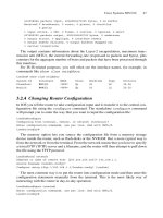
a RSVP-TE RESV message. The Explicit Route Object (ERO) allows RSVP-TE to spec-
ify a set of nodes that an RSVP-TE message has to traverse. Figure 14.12 shows sample
EROs modelled using the Loose and Strict (L/S) path constraint. A Strict hop indicates
that the next hop must be directly connected to the previous hop. The first example of
Figure 14.12 shows a set of strict hops that specify a path. A sequence of strict hops is
often used to nail down a path – that is, when the network administrator wants to enforce
a certain path. A Loose hop means that the node has to be present in the path before the
next hop, but does not have to be the next-hop. The second example of Figure 14.12
shows that only a subset of the nodes is listed in the ERO. With the Loose attribute, this
means that there is some room for re-routing this path. The path could potentially run
directly from Washington via Frankfurt to Pennsauken. In practice, the Loose option
causes more problems than it solves. The network is not in full control of the traffic path
anymore and in more complex topologies this may lead to strange results with long delay
paths. The third example in Figure 14.12 shows a mix between loose and strict hops. The
semantics of the ERO Objects allows for the combination of loose and strict hops in an
arbitrary fashion.
There are two general ways to create an ERO. The first is a manual specification and
the second, more sophisticated way, is automated computation. The manual configur-
ation will be discussed first.
You can configure a label switched path using an ERO in similar ways on IOS and
JUNOS. First you need to specify the ERO and next you need to link the ERO to a label
switched path.
IOS configuration
In IOS you can specify an ERO manually using the ip explicit-path statement. The
next-address specifies the next-element in the ERO. By default all hops in the ERO are
strict except when you supply the loose keyword.
ip explicit-path identifier name via-Penssauken enable
next-address 192.168.1.1
next-address loose 192.168.2.1

[…]
!
412 14. Traffic Engineering and MPLS
MPLS Signalling Protocols 413
Area 49.0001
Level 2-only
ERO
Paris strict;
Frankfurt strict;
London strict;
Pennsauken strict;
Area 49.0001
Level 2-only
ERO
Frankfurt loose;
Pennsauken loose;
Area 49.0001
Level 2-only
ERO
Frankfurt strict;
Pennsauken loose;
Pennsauken
Frankfurt
London
Washington
New York
Paris
Pennsauken
Frankfurt
London

Washington
New York
Paris
Pennsauken
Frankfurt
London
Washington
New York
Paris
FIGURE 14.12. The ERO consists of a mix and match list of Strict and/or Loose Hops
After defining the ERO you need to link it to an existing tunnel using the path-
option explicit argument to the tunnel mpls traffic-eng command.
IOS configuration
In order to switch from dynamic computation to an explicit execution use the tunnel mpls
traffic-eng path-option 5 explicit command.
interface Tunnel0
description TE Tunnel to Washington via Penssauken
ip unnumbered Loopback0
tag-switching ip
tunnel destination 192.168.20.1
tunnel mode mpls traffic-eng
tunnel mpls traffic-eng autoroute announce
tunnel mpls traffic-eng path-option 5 explicit name via-Penssauken
!
In JUNOS the configuration is very similar – first you specify the ERO.
JUNOS configuration
In JUNOS you configure manual EROs under the protocols mpls path {} configura-
tion branch.
protocols {
mpls {

path via-Penssauken {
192.168.1.1 strict;
192.168.2.1 loose;
}
}
}
Next you link the ERO into an existing label switched path. You need to declare the
path as a primary or secondary path.
JUNOS configuration
The tunnel is configured under the protocols mpls label-switched-path {} state-
ment. JUNOS has the notion of a primary/secondary path where you can specify a
backup path that is immediately used if the primary path fails.
protocols {
mpls {
label-switched-path “TE Tunnel to Washington via Pennsauken” {
to 192.168.20.1;
primary via-Pennsauken;
}
}
}
414 14. Traffic Engineering and MPLS
After you have configured your tunnels, you need to verify if the TE tunnel is up and if
the tunnel is following the desired path. Because awkward combination of the Loose and
Strict Hop option can cause unexpected results – the Record Route Object (RRO) pro-
vides better visibility for troubleshooting purposes. The Record Route Object is embed-
ded in the RSVP-TE RESV messages. During its journey from the egress router to the
ingress router all IP addresses are recorded and stored at the ingress router. On IOS, you
have to explicitly turn on generation to the RRO object using a Tunnel Interface path
option, in JUNOS it is automatic.
IOS configuration

In IOS the Record Route Object (RRO) is not automatically generated for a TE tunnel. It
needs to get configured explicitly using the tunnel mpls traffic-eng record-route
command.
interface Tunnel0
[… ]
tunnel mpls traffic-eng record-route
!
The contents of the RRO Object can be displayed using the show mpls traffic-
eng tunnels command in IOS.
IOS output
The show mpls traffic-eng tunnels command contains all the information around a
tunnel. The configured ERO, the tunnel’s bandwidth, outgoing labels and more of interest
is included in the Route Record Object (RRO).
London#show mpls traffic-eng tunnels
Name: TE Tunnel to Washington via Pennsauken (Tunnel0) Destination: 192.168.20.1
Status:
Admin: up Oper: up Path: valid Signalling: connected
path option 1, type explicit via-Pennsauken (Basis for Setup,path weight 10)
Config Parameters:
Bandwidth: 1 kbps (Global) Priority: 7 7 Affinity: 0x0/0xFFFF
Metric Type: TE (default)
AutoRoute: enabled LockDown: disabled Loadshare: 1 bw-based
auto-bw: disabled
InLabel : -
OutLabel : POS4/1, 100016
MPLS Signalling Protocols 415
RSVP Signalling Info:
Src 192.168.1.2, Dst 192.168.20.1, Tun_Id 0, Tun_Instance 511
RSVP Path Info:
My Address: 192.168.1.2

Explicit Route: 192.168.1.1 192.168.168.3
Record Route:
Tspec: ave rateϭ1 kbits, burstϭ1000 bytes, peak rateϭ1 kbits
RSVP Resv Info:
Record Route: 172.16.33.1 172.16.38.1
Fspec: ave rateϭ1 kbits, burstϭ1000 bytes, peak rateϭ1 kbits
History:
Tunnel:
Time since created: 12 days, 17 hours, 39 minutes
Time since path change: 1 minutes, 13 seconds
Current LSP:
Uptime: 1 minutes, 13 seconds
Most often you will notice a difference between the configured ERO and the recorded
PATH. It is common practice to use a router’s loopback ID as the address for a loose
hop. However, the route recorder in the PATH message thinks entirely in terms of link
addresses. So even if we used in our example the 192.168/16 addresses, the ones actually
reported back in the RRO are from the link-address space 172.16/16.
In JUNOS you can also display the recorded path using the show mpls lsp
ingress detail command.
JUNOS output
hannes@Frankfurt> show mpls lsp ingress detail
Ingress LSP: 1 sessions
192.168.1.1
From: 192.168.1.2, State: Up, ActiveRoute: 0, LSPname: to-Washington
ActivePath: (primary)
LoadBalance: Random
Encoding type: Packet, Switching type: Packet, GPID: IPv4
*Primary State: Up
Computed ERO (S [L] denotes strict [loose] hops): (CSPF metric: 20)
192.168.1.1 192.168.168.3 S

Received RRO (ProtectionFlag 1ϭAvailable 2ϭInUse 4ϭB/W 8ϭNode):
172.16.33.1 172.16.38.1
Total 1 displayed, Up 1, Down 0
JUNOS behaves similarly to IOS, where the Route Path Recording is done using link
addresses.
If you want to achieve any-to-any MPLS connectivity between all routers in your
network, then the consequence is to deploy a full-mesh of RSVP-TE tunnels. However,
there are severe scaling implications with that approach. To overcome these scaling
limitations a more lightweight MPLS label setup protocol called the Label Distribution
Protocol (LDP) is used.
416 14. Traffic Engineering and MPLS
14.4.3 LDP
LDP is defined in RFC 3036 and it describes a lean, lightweight protocol that brings up a
full-mesh of connectivity to all LDP speakers in the network. Generally, the term full-
mesh raises warning flags in every network engineer’s head due to the perceived scaling
problems. However, LDP uses a technique called label-merging which is very conserva-
tive with label allocation. Consider the right-hand side of Figure 14.13. There are five
drawings inside the figure, one for each possible egress router. The egress router is marked
with an E, and the metric on each link is 4.
MPLS Signalling Protocols 417
Frankfurt
Pa
LDP label allocation
6
4
4
4
4
4
6

4
4
4
4
4
6
4
4
4
4
4
6
4
4
4
4
4
6
4
4
4
4
4
RSVP label allocation
6
4
4
4
4
4

6
4
4
4
4
4
6
4
4
4
4
4
6
4
4
4
4
4
6
4
4
4
4
4
Frankfurt
London
Washington NewYork
Paris
E
E

Frankfurt
London
Washington New York
Paris
Frankfurt
London
Washington
NewYork
Paris
Frankfurt
London
Washington
NewYork
Paris
Frankfurt
London
Washington
New York
Paris
Frankfurt
London
Washington
New York
Paris
Frankfurt
London
Washington NewYork
Paris
Frankfurt
London

Washington NewYork
Paris
Frankfurt
London
Washington New York
Paris
Frankfurt
London
Washington
NewYork
Paris
E
E
E
E
E
E
E
E
FIGURE 14.13. LDP consumes less forwarding state per link than RSVP does
The figure describes the LSPs and the necessary forwarding state to set up full-mesh
connectivity between all five routers in the core network. Using RSVP-TE, we would
need at least N
*
(N – 1)/2 ϭ 10 explicitly configured tunnels. Because LDP supports label
merging, some labels can be re-used by other label switched paths. Unlike RSVP-TE,
LDP signals its label using a mode called downstream unsolicited, which means that
the labels are signalled from the egress router to the ingress router. Each LDP speaker
advertises prefixes according to the egress policy. In JUNOS, the default egress policy is
just to advertise the loopback IP address. The IOS default egress policy is to advertise both

the loopback and all the directly connected interfaces. Upstream nodes create MPLS
SWAP states and pass on the label-mapping message to their upstream nodes, which cre-
ate again MPLS SWAP states, and pass them on to further upstream nodes, and so on. The
resulting shape of the merged tree is called a sink tree. (In datacom speech the egress or
destination point is sometimes called the sink.) And because the root of the tree is at the
egress router, it is therefore a sink tree.
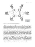
Figure 14.14 shows the number of forwarding entries (FE) that the sum of all label
switched paths generates. Even in the small topology, LDP behaves better than
RSVP-TE. LDP has an average of 3 FEs per link versus RSVP-TE, which consumes an
average of 4.33 FEs per link. LDP is therefore the protocol of choice for edge systems
like VPN and/or customer access routers, due to LDP’s ability to supply a full-mesh con-
nectivity to all the other LDP speakers with no setup complexity at all.
The configuration of LDP is a simple one: just enable it on a per-interface basis. An
LDP configuration for router London on IOS could look like the following:
IOS configuration
In IOS two configuration lines are necessary for running LDP. First turn on MPLS pro-
cessing on an interface plus the necessary Layer-2 Supporting Protocols like MPLSCP
over PPP using the tag-switching ip keyword. The mpls label protocol ldp key-
word tells the system to run LDP rather than TDP (Cisco’s proprietary predecessor
to LDP).
London#sh running-config
[… ]
!
interface POS4/1
ip address 172.17.0.5 255.255.255.252
ip router isis
encapsulation ppp
mpls label protocol ldp
tag-switching ip
!

Shortly after configuration, a remote LDP neighbour should be detected and an LDP
session is then set up automatically. You can verify the neighbour state using the show
mpls ldp neighbor operational level command.
418 14. Traffic Engineering and MPLS
419
Forwarding state/LDP label allocation
Forwarding state/RSVP label allocation
8 FE
4 FE
4 FE
4 FE
3 FE
3 FE
4 FE
2 FE
3 FE
3 FE
3 FE
3 FE
avg. 3 FE/LINK
avg. 4.33 FE/LINK
Frankfurt
London
Washington
New York
Paris
Frankfurt
London
Washington
New York

Paris
F
IGURE
14.14. The sum of all forwarding states show that LDP is more frugal than RSVP
IOS output
Under the show mpls ldp <*> hierarchy several commands are available to verify neigh-
bour state and timers.
London#show mpls ldp neighbor
Peer LDP Ident: 192.168.0.1:0; Local LDP Ident 192.168.13.8:0
TCP connection: 192.168.0.1.646 - 192.168.13.8.11000
State: Oper; Msgs sent/rcvd: 207/179; Downstream
Up time: 00:28:43
LDP discovery sources:
POS4/0, Src IP addr: 172.16.0.2
Addresses bound to peer LDP Ident:
172.16.0.2
The display output shows whether the session is up and what IP addresses are being
used. LDP uses link IP addresses for discovery and loopback IP addresses for session
setup. If a session does not come up due to addressing conflicts the output of this com-
mand is providing valuable information for troubleshooting.
In JUNOS we need to make sure that family mpls is configured under the logical
interface branch. In addition we add a list of interfaces where we want to speak LDP
under the protocols ldp stanza.
JUNOS configuration
In JUNOS you need to specify the interface where you want to run LDP both under the
protocols mpls {} and protocols ldp {} stanza. Alternatively you can set the mpls
interface list to all which allows allocation of labels on all interfaces. In addition every
logical interface needs to have the family mpls configured.
hannes@Frankfurt# show
[… ]

interface ge-0/0/0 {
unit 0 {
family mpls;
}
}
protocols {
mpls {
interface all;
}
ldp {
interface so-0/1/2.0;
}
}
[… ]
It remains unknown why mpls interface all {} is not the default option,
since this does not break anything by being turned on. On the other hand, it does break
420 14. Traffic Engineering and MPLS
proper label allocation if the interfaces are not listed under this command hierarchy. Not
all default decisions are obvious.
The neighbour state is verified using the show ldp neighbor command.
JUNOS output
You can verify the neighbour state using the show ldp neighbor detail operational
level command.The output displays the session IP addresses plus the neighbour’s link IP
address.
hannes@Frankfurt> show ldp neighbor detail
Address Interface Label space ID Hold time
10.0.0.5 so-0/1/2.0 62.154.13.8:0 11
Transport address: 62.154.13.8, Configuration sequence: 0
Up for 01:33:30
LDP is very much dependent on a working IGP. LDP itself cannot be run in stand-

alone mode. Like BGP it is topology agnostic and cannot assert which label is better over
another. LDP picks the label of the outgoing interface based on the best IGP distance. If
the LDP topology is non-congruent than the IGP topology then LDP paths might get
black holed.
One of the most frequent configuration mistakes is that the list of interfaces that run IS-IS
and the list of interfaces which run LDP are not the same. Consider Figure 14.15. All links
in the core network have IS-IS and LDP enabled, except the link between Washington and
New York, which lacks LDP due to a configuration mistake. Paris learns the /32 FEC of the
New York router via the London, Frankfurt, Washington path and selects the path via
Washington because it is on the shortest path tree. The traffic gets labelled to Washington
where it gets black holed because no valid MPLS labelled switched paths to the FEC of
New York are available.
MPLS Signalling Protocols 421
10 IS-IS
LDP
4 IS-IS
LDP
12 IS-IS
4 IS-IS
LDP
4 IS-IS
LDP
Frankfurt
London
Washington NewYork
Paris
4 IS-IS
LDP
FIGURE 14.15. If the IS-IS and LDP topology is non-congruent Washington is black holing traffic
If you are troubleshooting an MPLS reachability problem, the first thing to check is if

the IS-IS adjacencies match the LDP session. It remains problematic why router vendors
do not change their default behaviour. LDP should be automatically brought up as soon
as you enable IS-IS on an interface. If someone does not want to run LDP, they could
then explicitly turn it off. That way you can prevent a network from black holing traffic.
14.4.4 Conclusion
Clients often ask what the “signalling protocol of choice” is. In 99 per cent of the cases,
the answer is: both (LDP and RSVP-TE). Both protocols augment each other. LDP lacks
path control, however. It is very frugal in its label usage and therefore inherently scalable.
RSVP-TE is a heavyweight both from an administrative point of view as well as from a
label allocation perspective; however, RSVP-TE has sound path control properties. So in
general, networks use LDP, but once they need to offload some traffic from hot trunks,
they use RSVP-TE in addition. There is no need to build full-mesh, explicitly configured
RSVP-TE tunnels. First, pick a careful IGP metric scheme that provides good-enough
routes, and then on top of that use RSVP-TE established TE-tunnels to take some heat off
the hot trunks.
14.5 Complex Traffic Engineering by CSPF Computations
Traffic engineering is deployed in two general ways: the first option is when the network
administrator wants to have the maximum level of control and explicitly configures all the
label switched paths, plus the EROs. In moderately complex topologies, however, manu-
ally writing up tens to hundreds of EROs is a daunting task and almost certainly over-
whelms the processing capabilities of humans. This is especially true if constraints like
hop count and backup path diversity need to be considered; in these cases, automatic com-
putation of EROs is the preferred choice. The computation of the EROs is done using a
distributed traffic engineering database called the TED. The contents of this database are
carried in IS-IS or OSPF. Figure 14.16 shows the differences between the two models.
422 14. Traffic Engineering and MPLS
Extended IS-IS
Routing Table
Traffic Engineering
Database (TED)

Constrained
Shortest Path First
(CSPF)
User constraints
ERO
RSVP Signalling
2
1
FIGURE 14.16. The RSVP Call Manager gets its input from the outcome of the CSPF calculation
which is influenced by User Constraints and Topological Input
In the first method, the network administrator supplies the ERO data, and in the second the
EROs are calculated using a Constrained Shortest Path First Calculation (CSPF) based on
user constrained TED input from the routers. The final result is an ERO which gets passed
to RSVP-TE for LSP setup.
You can display the contents of the TED database using the show mpls traffic-
eng topology command in IOS and show ted database extensive com-
mand in JUNOS.
IOS command output
London#show mpls traffic-eng topology
My_System_id: 1921.6800.1008.00 (isis level-2)
Signalling error holddown: 10 sec Global Link Generation 5
IGP Id: 1921.6800.1012.00, MPLS TE Id:192.168.0.12 Router Node (isis level-2)
link[0]: Point-to-Point, Nbr IGP Id: 1921.6800.1008.00, nbr_node_id:1, gen:2
frag_id 0, Intf Address:172.16.0.2, Nbr Intf Address:172.16.0.1
TE metric:10, IGP metric:10, attribute_flags:0x0
physical_bw: 2488320 (kbps), max_reservable_bw_global: 2488320 (kbps)
max_reservable_bw_sub: 0 (kbps)
Global Pool Sub Pool
Total Allocated Reservable Reservable
BW (kbps) BW (kbps) BW (kbps)

bw[0]: 0 2488320 0
bw[1]: 0 2488320 0
bw[2]: 0 2488320 0
bw[3]: 0 2488320 0
bw[4]: 0 2488320 0
bw[5]: 0 2488320 0
bw[6]: 0 2488320 0
bw[7]: 0 2488320 0
The TED database contains all IP addresses, links and current bandwidth reservation
states. The data found here is the foundation for the CSPF calculation which produces a
path described by an ERO.
JUNOS command output
hannes@Frankfurt> show ted database extensive
TED database: 3 ISIS nodes 3 INET nodes
NodeID: Frankfurt.00(192.168.0.8)
Type: Rtr, Age: 189 secs, LinkIn: 1, LinkOut: 1
Protocol: IS-IS(2)
To: London.00(192.168.0.8), Local: 172.16.0.1, Remote: 172.16.0.2
Color: 0 <none>
Metric: 10
Static BW: 2488.32Mbps
Reservable BW: 2488.32Mbps
Complex Traffic Engineering by CSPF Computations 423
Available BW [priority] bps:
[0] 2488.32Mbps [1] 2488.32Mbps [2] 2488.32Mbps [3] 2488.32Mbps
[4] 2488.32Mbps [5] 2488.32Mbps [6] 2488.32Mbps [7] 2488.32Mbps
Interface Switching Capability Descriptor(1):
Switching type: Packet
Encoding type: Packet

Maximum LSP BW [priority] bps:
[0] 2488.32Mbps [1] 2488.32Mbps [2] 2488.32Mbps [3] 2488.32Mbps
[4] 2488.32Mbps [5] 2488.32Mbps [6] 2488.32Mbps [7] 2488.32Mbps
Why isn’t the data for CSPF calculations taken straight from the link-state database of
the routing protocol? Well, there still may be OSPF deployed in parts of the network. The
TED is a unified view to the topology of the network, so no matter which IGP (OSPF,
IS-IS, or even vendor-proprietary protocols) supplied the topology data. The TED is a
unified, abstracted view and knows only about nodes, links and link attributes.
How does IS-IS generate and encode the data in the TED output? How does it know
that a certain interface is an OC-48 interface? As soon as RSVP-TE is enabled on an
interface, a lot of extra information is generated and conveyed using IS-IS.
Consider the following tcpdump output of a LSP before RSVP-TE has been
turned on.
Tcpdump output
If RSVP-TE is not enabled on a core interface then no bandwidth relevant information is
generated inside the Extended IS Reach TLV.
00:27:20.871975 OSI, IS-IS, length: 104
L2 LSP, hlen: 27, v: 1, pdu-v: 1, sys-id-len: 6 (0), max-area: 3 (0)
lsp-id: 0620.0000.0001.00-00, seq: 0x00000030, lifetime: 1196s
chksum: 0x1d9d (correct), PDU length: 104, L1L2 IS
Area address(es) TLV #1, length: 4
Area address (length: 3): 49.0001
Protocols supported TLV #129, length: 1
NLPID(s): IPv4
Traffic Engineering Router ID TLV #134, length: 4
Traffic Engineering Router ID: 62.0.0.1
IPv4 Interface address(es) TLV #132, length: 4
IPv4 interface address: 62.0.0.1
Hostname TLV #137, length: 9
Hostname: Frankfurt

Extended IS Reachability TLV #22, length: 23
IS Neighbor: 0621.5401.3008.00, Metric: 10, sub-TLVs present (12)
IPv4 interface address subTLV #6, length: 4, 10.0.0.2
IPv4 neighbor address subTLV #8, length: 4, 10.0.0.1
Extended IPv4 Reachability TLV #135, length: 18
IPv4 prefix: 62.0.0.1/32, Distribution: up, Metric: 0
IPv4 prefix: 10.0.0.0/30, Distribution: up, Metric: 10
424 14. Traffic Engineering and MPLS
Complex Traffic Engineering by CSPF Computations 425
Next, traffic engineering and RSVP-TE is configured on IOS and JUNOS and the
resulting LSP structure is examined.
IOS configuration
In IOS you need to enable traffic-eng globally and under the router isis stanza.
Additionally you need to enable it on each interface using the mpls traffic-eng tunnels
command plus the ip rsvp bandwidth keyword specifies how much bandwidth can be
reserved.
London#sh running-config
[… ]
mpls traffic-eng tunnels
!
interface POS4/1
[… ]
ip router isis
mpls traffic-eng tunnels
tag-switching ip
ip rsvp bandwidth 2488320 2488320
!
router isis
mpls traffic-eng router-id Loopback0
mpls traffic-eng level-2

metric-style wide level-2
[… ]
!
The ip rsvp bandwidth statement takes two parameters. The first is the max-
imum amount of bandwidth that is reservable on the interface, and the second is the max-
imum amount of bandwidth that is available for a single reservation. Typically those two
values are the same, which means that a single reservation can eat up all the interface’s
bandwidth. Under the router isis stanza you need to specify the IS-IS level to which
you want to send traffic engineering information. Unfortunately, you need to decide for
Level-1 or Level-2. Both levels are not yet supported. Typically Level-2 is configured, and
that is done here.
In JUNOS the sending of traffic engineering sub-TLV parameters is the default behav-
iour and there is no need to configure any further global options. All that needs to be con-
figured is to add the interface under the protocols rsvp stanza.
JUNOS configuration
In JUNOS you need to specify the interface where you want to send bandwidth and reser-
vation state both under the protocols mpls {} and protocols rsvp {} stanza.
Alternatively you can set the mpls interface list to all. You can change the
426 14. Traffic Engineering and MPLS
oversubscription of RSVP bandwidth by changing the default value of 100% using the
subscription keyword.
hannes@Frankfurt# show
[… ]
protocols {
mpls {
interface all;
}
rsvp {
interface so-0/1/2.0 {
subscription 120;

}
}
}
[… ]
As soon as you enable RSVP-TE on an interface on which the router has established
an adjacency, then the LSP gets updated with a lot of extra information, encoded by
adding several sub-TLVs to the extended IS Reachability TLV #22.
Tcpdump output
An RSVP-TE enabled IS-IS adjacency shows the interface speed plus current reservation
state using 8 pre-emption classes.
00:28:20.760649 OSI, IS-IS, length: 156
hlen: 27, v: 1, pdu-v: 1, sys-id-len: 6 (0), max-area: 3 (0), pdu-type: L2 LSP
lsp-id: 0620.0000.0001.00-00, seq: 0x00000031, lifetime: 1196s
chksum: 0x2674 (correct), PDU length: 156, L1L2 IS
Area address(es) TLV #1, length: 4
Area address (length: 3): 49.0001
Protocols supported TLV #129, length: 1
NLPID(s): IPv4
Traffic Engineering Router ID TLV #134, length: 4
Traffic Engineering Router ID: 62.0.0.1
IPv4 Interface address(es) TLV #132, length: 4
IPv4 interface address: 62.0.0.1
Hostname TLV #137, length: 9
Hostname: Frankfurt
Extended IS Reachability TLV #22, length: 75
IS Neighbor: 0621.5401.3008.00, Metric: 10, sub-TLVs present (64)
IPv4 interface address subTLV #6, length: 4, 10.0.0.2
IPv4 neighbor address subTLV #8, length: 4, 10.0.0.1
Unreserved bandwidth subTLV #11, length: 32
priority level 0: 2488.320 Mbps

priority level 1: 2488.320 Mbps
priority level 2: 2488.320 Mbps
priority level 3: 2488.320 Mbps
Complex Traffic Engineering by CSPF Computations 427
priority level 4: 2488.320 Mbps
priority level 5: 2488.320 Mbps
priority level 6: 2488.320 Mbps
priority level 7: 2488.320 Mbps
Reservable link bandwidth subTLV #10, length: 4, 2488.320 Mbps
Maximum link bandwidth subTLV #9, length: 4, 2488.320 Mbps
Administrative groups subTLV #3, length: 4, 0x00000000
Extended IPv4 Reachability TLV #135, length: 18
IPv4 prefix: 62.0.0.1/32, Distribution: up, Metric: 0
IPv4 prefix: 10.0.0.0/30, Distribution: up, Metric: 10
Figure 14.17 shows the contents of the Traffic Engineering Router ID TLV #134. It
basically contains a single unique 32-bit ID in order to uniquely identify a router in the
TED. The TE Router ID TLV #134 corresponds to the OSPF Router-ID and puts the
topology gathered by the two protocols into a relationship in the TED. The underlying
problem is that IS-IS identifies its nodes through System-IDs (48-bit) and OSPF does it
using Router-IDs (32-bit). By issuing a TLV #134 the IS-IS speaker tells other routers
what would be the corresponding OSPF router-ID in case one router is running both
OSPF and IS-IS for transition purposes.
In Table 14.2 there is a list of sub-TLVs to the extended Reachability TLV #22. These
are used for conveying various pieces of link information like Admin (Affinity) Groups,
bandwidth parameters and IPv4 endpoint addresses. Chapter 11 “TLVs and Sub-TLVs”
explores more about TLVs and sub-TLV nesting.
TLV Type
TLV Length
Traffic engineering router ID
132

Bytes
1
1
4
4
FIGURE 14.17. The Traffic Engineering TLV #134 contains a unique ID which identifies a TE
speaker throughout disjoint TE domains
TABLE 14.2. Sub-TLV code points.
Sub-TLV Sub-TLV name
3 Administrative (Affinity) Group
4 Link Local ID
5 Link Remote ID
6 IPV4 Interface Address
8 IPV4 Remote Interface Address
9 Maximum Link Bandwidth
10 Reserve Able Bandwidth
11 Unreserved Bandwidth
18 TE-Metric
20 Link Protection Type (GMPLS)
21 Switching Capability (GMPLS)
Not yet assigned by IANA Bandwidth Constraints
428 14. Traffic Engineering and MPLS
After the TED has been populated with the above link-related information, the routers
engage in a CSPF calculation based on the network operator’s constraints. The CSPF is
a two-pass calculation where in the first pass all the links that do not fit a certain con-
straint are removed, and the second pass is a vanilla SPF calculation as was described in
Chapter 10, “SPF and Route Calculation”.
See Figure 14.18 for an example of CSPF. The network needs to compute a label
switched path between Washington and New York which can only run on links carrying
the “Internet” Link Colour (Affinity Group) and must not run on links carrying the

“Maintenance” Link Colour (Affinity Group). The amount of reserved bandwidth is
600 MBit/s. In the first pass of the CSPF calculation all the links that do not belong to the
required “Internet” administrative group are removed. The direct link between Washington
and New York does not fit the constraint because it carries the “Maintenance” Link Colour.
Next, all the links that do not have sufficient bandwidth are removed. The reservation of
additional 600 MBit/s would oversubscribe the link between Washington and Frankfurt and
is removed as well.
Based on the resulting “skeleton”, the routers run an SPF calculation and try to find the
shortest path node between the source and the destination point. In our example, the path
via Paris, Frankfurt and London fits all the constraints and therefore the tunnel comes up.
The result of the SPF calculation does not really matter because in this case there is only
a single path left which fulfils all constraints.
If there are too many constraints during the first pass and there are no feasible paths at
all, then the result of the SPF calculation will be that there is no shortest path between a
pair of nodes. Note that in CSPF calculations, there is not any type of crank-back proced-
ure where the systems try to find a path at all costs. This was common practice for voice
networks, but crank-back schemes run the risk of sending traffic around the continent sev-
eral times, like the overlay networks of the 1990s did. Sometimes the result of the CSPF
calculation is even no result at all and then no tunnel will be signalled.
14.6 LDP over RSVP-TE Tunnelling
Which signalling protocol (LDP or RSVP-TE) to use is one of the first questions that net-
work operators raise when deploying MPLS. Many people like the “call-oriented” notion
of RSVP-TE and the amount of control the network operator has over traffic. On the other
hand, LDP works like a charm – you turn it on and seconds later you have got label
switched paths to every corner of your network at almost no cost and with nice scaling
properties. To achieve the same connectivity matrix that LDP creates, one would have to
deploy RSVP-TE in a full-mesh fashion with a dedicated tunnel between all the MPLS
edge routers. In moderate size networks full-mesh RSVP-TE may be a design choice, how-
ever, in medium-to large-sized networks, this may be a scaling nightmare. Recall that in a
full-mesh network with 1000 edge routers, one would need 1000

*
(1000 – 1)/2 ϭ 499,500
label switched paths! The refresh noise alone from repeating each reservation every 30 sec-
onds, which will be processed twice (PATH and RESV messages from all the core routers
along the label switched path), would result in approximately 30,000 messages per second
being processed by each core router. Although there are extensions to aggregate refreshes
LDP over RSVP-TE Tunnelling 429
0 MBit/s rsvd.
Internet, Maintenance
400 MBit/s rsvd.
Internet
280 MBit/s rsvd.
Internet
1900 MBit/s rsvd.
Internet
1250 MBit/s rsvd.
Internet
1100 MBit/s rsvd.
Internet
4
4
6
4
4
4
400 MBit/s rsvd.
Internet
280 MBit/s rsvd.
Internet
1900 MBit/s rsvd.

Internet
1250 MBit/s rsvd.
Internet
1100 MBit/s rsvd.
Internet
4
4
4
4
4
Prune all links that do not have Internet and Maintenance set
1
Prune all links that do not fit Bandwidth requirements
2
280 MBit/s rsvd.
Internet
4 4
1100 MBit/s rsvd.
Internet
4
1250 MBit/s rsvd.
Internet
Frankfurt
London
Washington New York
Paris
Frankfurt
London
Washington
New York

Paris
Frankfurt
London
Washington New York
Paris
400 MBit/s rsvd.
Internet
4
FIGURE 14.18. In the CSPF calculation all paths that do not meet any of the constraints are pruned
off the final topology
430 14. Traffic Engineering and MPLS
LDP
RSVP
POP
POP
POP
POP
POP
LDP over RSVP tunneling
3
Frankfurt
London
Washington
NewYork
Paris
TE Tunnel
2
1
FIGURE 14.19. Traffic from Paris to London does not take the TE tunnel path
(see RFC 2961 for details), and thereby reduce the refresh noise, the underlying problem

(which is the familiar networking “N^2” problem) is not addressed by aggregation alone.
For scalability reasons, network operators are tempted to use the more scaleable LDP,
which sets up a kind of full-mesh matrix (based on sink trees). But LDP label selection is
dictated by the IGP, and that translates to a lack of traffic path-control because no one wants
to tweak IGP metrics anymore.
So the answer to the signalling protocol question is most often to use both protocols
where they fit best. LDP is used for setting up lightweight labels switched paths across
the network, and RSVP-TE is used for traffic engineering.
Consider Figure 14.19, where both protocols are deployed. LDP is deployed across
the core for establishing label switched paths between all routers in the network (1).
Additionally, there is a Traffic Engineering Tunnel between the core router in Paris and
London (2). If traffic is loaded on that path, then all the traffic will be guided through
LDP paths and the single RSVP-TE TE tunnel in the core is completely ignored. Why?
Because MPLS is a source routing technique. The ingress router makes the choice as to
which label switched path is used for traffic forwarding. If an edge (ingress) router does
not know about a TE tunnel path in the core, then it will not use it.
The trick is now to make LDP use the TE tunnel in the core for forwarding. A tech-
nique called LDP over RSVP-TE tunnelling is used for that purpose. Previously, LDP
was deployed in a hop-by-hop fashion – the LDP speakers propagate their label mapping
messages from node to adjacent node. In order to make LDP use the TE tunnel, an add-
itional LDP session is brought up between the Paris and London core router (3). For set-
ting up a session between a pair of non-adjacent routers, an LDP option called targeted
Hellos is used. Targeted Hellos are similar to internal BGP sessions. The two LDP speak-
ers at the edge send a Hello across several hops. If the two speakers at the edge agree on
the capabilities reported in the Hello message, then an LDP session (using TCP) is estab-
lished to advertise label mappings. All label advertisements learned via the multi-hop
LDP over RSVP-TE Tunnelling 431
LDP session are now associated with the TE tunnel and then used for traffic forwarding.
When Paris advertises a label back to its local POP routers, then a SWAP/PUSH state on
the forwarding plane is generated. The label of the TE tunnel is PUSHed as top level

label and the label learned via the multi-hop LDP session is the SWAPed label. The edge
routers send their traffic down the LDP established paths and do not even know that their
traffic is being engineered in the core topology. As soon as the traffic arrives at the
ingress of the TE tunnel (Paris), an additional label is PUSHed on top of the label stack
and the traffic is sent down the TE tunnel. The penultimate TE tunnel router (New York)
removes the top label and the LDP label underneath becomes visible and is used for fur-
ther relaying traffic towards the LDP egress router.
Configuration of LDP over RSVP-TE tunnelling is done using the mpls ldp
neighbor <address> targeted ldp keyword in IOS and the ldp-tunneling
keyword in JUNOS.
IOS configuration
In IOS LDP tunnelling is a global option which can be configured using the mpls ldp
neighbor <address> targeted statement.
London# show running-config
[… ]
mpls ldp neighbor 192.168.1.1 targeted ldp
[… ]
!
If the multi-hop LDP session comes up and there is an RSVP-TE tunnel to this des-
tination, then the resolver will automatically set up the SWAP/PUSH state. In JUNOS
LDP over RSVP-TE tunnelling is a property of the TE tunnel and is configured under the
protocols mpls label-switched-path <name> {} stanza.
JUNOS configuration
In JUNOS the ldp-tunneling keyword automatically sets up a session between two
ends of a TE tunnel.
[edit]
hannes@Frankfurt# show
[… ]
protocols {
mpls {

label-switched-path to-London {
to 192.168.0.8;
ldp-tunneling;
}
interface so-1/2/0;
interface l00.0;
}
[… ]
432 14. Traffic Engineering and MPLS
It is imperative that the loopback interface lo0.0 or interface all is listed when config-
uring LDP tunnelling. LDP multi-hop sessions are sourced using the IP address of the
lo0.0 interface. If it is not listed, then the tunnelled LDP session stays down.
LDP over RSVP-TE tunnelling is a good example of how label stacking contributes to
better scalability of the network. The LDP over RSVP-TE tunnelling example just needed
to set up one additional forwarding state at the TE tunnel ingress router. The rest of the
core topology was unaffected by the LDP tunnelling change. An additional advantage of
the clear layering is that once the tunnel goes down, immediately alternate paths (that is,
the LDP-only paths that are available) are available. Also, the churn for changing the label
state is almost zero, because only the TE ingress routers need to change forwarding state
to use the IGP guided paths.
Unfortunately LDP over RSVP-TE tunnelling does not solve the label selection issue
for all topologies. Typically, it only attracts traffic being sourced from directly attached
routers in the POP. For any edge router that is at least 2 hops upstream, it is not possible
to force traffic onto a certain path. Figure 14.20 illustrates the problem.
The links from Paris to Washington, Washington to New York, and Paris to Frankfurt
are congested. Frankfurt and Paris are major traffic sources. There is a TE tunnel between
Frankfurt and New York (1) – LDP tunneling is turned on. Now, all the Frankfurt POP
traffic is using the tunnel. What would be best is to also attract the traffic from Paris.
But this is not possible in this topology because Paris selects the label switched path to
New York via Washington, which is the shortest path.

In this simple topology the easiest fix would be to install another TE tunnel from Paris
to New York. However, in complex topologies, often the administrative overhead of man-
aging several local tunnels outweighs the convenience of having fewer tunnels to manage.
It would be nice if there was a tool where networks could gradually suck traffic to the
RSVP
2
1
LDP
POP
POP
POP
POP
POP
Frankfurt
London
Washington
NewYork
Paris
120% load
95% load
25% load4
4
4
6
4
1-10
30% load
20% load
110% load4
2

FIGURE 14.20. For traffic engineering of upstream routers forwarding adjacencies need to be
configured
LDP over RSVP-TE Tunnelling 433
head-end of a TE tunnel. But to affect non-local forwarding decisions, the network needs
to find a way to modify the route computation. And there is one. Forwarding adjacencies
are a way of re-advertising a label switched path in the IS-IS database.
14.7 Forwarding Adjacencies
The Edge MPLS routers, which speak LDP, have to rely on the IGP (IS-IS) to find the
shortest path to the destination. Recall that the general problem of traffic engineering is that
the shortest path is not always the best path. The tunnel must be made somewhat attractive
to the edge systems’ traffic. One way of doing this is to model the core TE tunnel as a direct
link and make the tunnels cost a little better than the resulting IGP cost. Because of that
slight difference, the edge systems will prefer to load traffic onto the tunnel.
A decade ago it was common to run IGPs over a tunnel. But running dynamic routing
protocols over a tunnel is almost always a recipe for disaster. Things behave really badly
if the total IGP cost over the tunnel undermines the total topologies’ cost. What happens
next is that the tunnel “wraps” around itself, ultimately causing a meltdown of the entire
network. Having those glorious meltdowns in mind, designers put a few restrictions on
re-advertising a TE tunnel as part of the IS-IS topology. First of all, no IS-IS Hellos are sent
down a tunnel. The router considers this forwarding adjacency to be up when the tunnel is
up. If there is a change in topology and the tunnel goes down, then the forwarding adja-
cency will go down as well. Because no Hellos are sent down the tunnel there is no infin-
ite recursion problem as there was when tunnelling IGPs in the 1990s. Still, there are
some things to watch out for. If the cost of the forwarding adjacency becomes too low
(that is, more attractive to the rest of the topology) then too much traffic is sucked towards
that tunnel. This could even totally mess up the IGP routing.
Reconsider Figure 14.20. If the TE tunnel is advertised with IS reach information in
the IS-IS database, then it seems as if there is now a direct, additional link between
Frankfurt and New York (2). The nice thing is that the metric of this “virtual” adjacency
can be configured arbitrarily. It can be set to a metric of 10, which makes the link totally

unattractive because there are shorter paths available. However, if the forwarding adja-
cency metric is set (for instance) to 1, then even non-local traffic is sucked into the tun-
nel, including all the POP traffic from (for example) Paris. Depending on the IGP metric
design, the power of forwarding adjacencies can do severe damage to the network.
Consider the IGP metric proposal in Figure 12.10. A metric of 1 is not used today, mainly
to leave some headroom for high speed links like OC768/STM-256 pipes. But if the
advertised metric of the tunnel is 1, even regional traffic between cities can be sucked
across the Atlantic. A common design rule is to keep the IGP cost slightly above the cost
of the real topology, and it should not exceed the typical link-metric inside the POP. The
idea is to suck the entire POP destinations across the tunnel, but keep the sucking-
distance low enough not to affect other region’s traffic.
In IOS forwarding adjacencies are a property of a TE tunnel and can be configured
using the tunnel mpls traffic-eng forwarding-adjacency parameter in
the tunnel interface configuration.
434 14. Traffic Engineering and MPLS
IOS configuration
In IOS you need to tell the tunnel interface that it has to re-advertise the TE tunnel into IS-
IS using the tunnel mpls traffic-eng forwarding-adjacency statement.
Additionally the resulting IS-IS metric needs to be specified using the regular isis
metric <*> statement.
London# show running-config
[… ]
interface Tunnel0
mpls traffic-eng tunnels
tag-switching ip
tunnel mode mpls traffic-eng
tunnel mpls traffic-eng forwarding-adjacency
isis metric 200 level-2
!
In JUNOS, a forwarding adjacency is an IS-IS property and is configured under the

protocols isis label-switched-path {} stanza.
JUNOS configuration
In JUNOS you need to reference a valid label switched path which needs to exist under
the protocols mpls {} stanza plus the IS-IS level and metric.
hannes@Frankfurt> show configuration
[… ]
protocols {
isis {
[… ]
label-switched-path Paris-to-London {
level 2 metric 200;
}
}
}
[… ]
How do the other routers know that an IS-IS adjacency is real (over physical links) or the
result of a forwarding adjacency (over a TE tunnel)? In order not to run into recursive tun-
nel loop problems, there is a differentiation. If you consider the tcpdump output, then you
can easily see the difference between a physical link adjacency and a forwarding adjacency.
Tcpdump output
A forwarding adjacency enabled IS reachability information does not carry any traffic engi-
neering sub-TLVs.
00:28:20.760649 OSI, IS-IS, length: 156
hlen: 27, v: 1, pdu-v: 1, sys-id-len: 6 (0), max-area: 3 (0), pdu-type: L2 LSP
lsp-id: 1921.6800.1014.00-00, seq: 0x0000df31, lifetime: 1196s
chksum: 0x2674 (correct), PDU length: 156, L1L2 IS
[… ]
Hostname TLV #137, length: 5
Hostname: Paris
Extended IS Reachability TLV #22, length: 86

physical link → IS Neighbor: 1921.6800.1008.00, Metric: 10, sub-TLVs present (64)
IPv4 interface address subTLV #6, length: 4, 172.16.0.2
IPv4 neighbor address subTLV #8, length: 4, 172.16.0.1
Unreserved bandwidth subTLV #11, length: 32
priority level 0: 2488.320 Mbps
priority level 1: 2488.320 Mbps
priority level 2: 2488.320 Mbps
priority level 3: 2488.320 Mbps
priority level 4: 2488.320 Mbps
priority level 5: 2488.320 Mbps
priority level 6: 2488.320 Mbps
priority level 7: 2488.320 Mbps
Reservable link bandwidth subTLV #10, length: 4, 2488.320 Mbps
Maximum link bandwidth subTLV #9, length: 4, 2488.320 Mbps
Administrative groups subTLV #3, length: 4, 0x00000000
Forw. Adjacency → IS Neighbor: 1921.6800.1012.00, Metric: 200, no sub-TLVs present
Extended IPv4 Reachability TLV #135, length: 18
IPv4 prefix: 62.0.0.1/32, Distribution: up, Metric: 0
IPv4 prefix: 172.16.0.0/30, Distribution: up, Metric: 10
The forwarding adjacency gets advertised as simply Extended IS Reach Adjacency
with no sub-TLVs at all attached to it. Therefore, the adjacency does not get moved to the
TED. It is almost as if this virtual “link” does not exist for the TED. If a link does not exist
in the TED, then no adjacency can be established over it, and the tunnel recursion prob-
lem is fixed. One of the key concepts of forwarding adjacencies is that the resulting vir-
tual link should always be worse than a real link. Chapter 17, “Future of IS-IS”, will
extend the forwarding adjacency concept to several switching layers and examine how
forwarding adjacencies can be utilized for G-MPLS applications.
Forwarding adjacencies are a nice tool to offload traffic from the shortest path with
minimal configuration and maximum impact. However, one problem remains: if the
path’s physical characteristics change, the delay characteristics of that path may also

change. In order to modify traffic paths for only some classes of traffic, DiffServ Traffic
Engineering needs to be deployed.
14.8 DiffServ Aware Traffic Engineering
Originally, traffic engineering was used to offload just best-effort traffic. This was fine,
because at that time, only best-effort traffic was routed. In recent years, however, there has
Forwarding Adjacencies 435