Microeconomics for MBAs - Chapter 15 pps

CHAPTER 15

Competitive and Monopsonistic
Labor Markets

Labour, like all other things which are purchased and sold, and which may be increased
or diminished in quantity, has its…market price
David Ricardo

rofessional football players earn more than ministers or nurses. Social workers
with college degrees generally earn less than truck drivers, who may not have
completed high school. Professors of accounting typically earn more than
professors of history with equivalent educational background and teaching experience.
Even if your history professor is an outstanding teacher, capable of communicating
effectively and concerned about students’ problems, she probably earns less than a
mediocre teacher of accounting.
Why do different occupations offer different salaries? Obviously not because of
their relative worth to us as individuals. Just as there is a market for final goods and
services—calculators, automobiles, dry cleaning—there is a market for labor as a
resource in the production process. In this competitive labor market, the forces of supply
and demand determine the wage rate workers receive.
By concentrating on the economic determinants of employment—those that relate
most directly to production and promotion of a product—we do not mean to suggest that
other factors are unimportant. Many noneconomic forces influence who is employed at
what wage, including social status, appearance, sex, race, and personal acquaintances.
Our purpose is simply to show how economic forces affect the wages paid and the
number of employees hired. Such a model can show not only how labor markets work,
but how attempts to legislate wages, like minimum wage laws, affect the labor market.
The general principles that govern the labor market also apply to the markets for
other resources, principally land and capital. The use of land and capital has a price,
called rent or interest, which is determined by supply and demand. Furthermore, land,

capital, and labor are all subject to the law of diminishing marginal returns. Beyond a
certain point and given a fixed quantity of at least one resource, more land, labor, or
capital will produce less and less additional output.


The Demand for and Supply of Labor
Labor is a special kind of commodity, one in which people have a personal stake. The
employer buys this commodity at a price: the wage rate the laborer receives in exchange
P
Chapter 15 Competitive and Monopsonistic
Labor Markets



2

for his or her efforts. In a competitive market, the price, or wage rate, of labor is
determined just as other prices are, by the interaction of supply and demand. To
understand why a person earns what he does, then, we must first consider the
determinants of the demand and supply of labor.

The Demand for Labor
The demand for labor is the assumed inverse relationship between the real wage rate
and the quantity of labor employed during a given period, everything else held constant.
The demand curve for labor generally slopes downward. At higher wage rates,
employers will hire fewer workers than at lower wage rates.
The demand for labor is derived partly from the demand for the product produced.
If there were no demand for mousetraps, there would be no need—no demand—for
mousetrap makers. This general principle applies to all kinds of labor in an open market.
Plumbers, textile workers, and writers can earn a living because there is a demand for the

products and services they offer. The greater the demand for the products and the greater
the demand for the labor needed to produce it and the greater the demand for a given
kind of labor, everything else held equal, the higher the wage rate.
The productivity of labor that is, the quantity of work a laborer can produce in a
given unit of time—is another critically important determinant of the demand for labor.
The price of the final product puts a value on a laborer’s output, but her productivity
determines how much she can produce. Together, labor productivity and the market
price of what is produced determine the market value of labor to employers, and
ultimately the employers’ demand for labor.
We can predict that the demand for labor will rise and fall with increases and
decreases in both productivity and product price. Suppose, for example, that mousetraps
are sold in a competitive market, where their price is set by the interaction of supply and
demand. Assume also that mousetrap production is subject to diminishing marginal
returns. As more and more units of labor are added to a fixed quantity of plant and
equipment, output expands by smaller and smaller increments.
Column 2 of Table 15.1 illustrates diminishing returns. The first laborer
contributes a marginal product—or additional output—of six mousetraps per hour. From
that point on, the marginal product of each additional laborer diminishes. It drops from
five mousetraps to four to three and so on, until an extra laborer adds only one mousetrap
to total hourly production.
The employer’s problem, once production has reached the range of marginal
diminishing returns, is to determine how many laborers to employ. She does so by
considering the value of the marginal product of labor. Column 3 shows the market price
of each mousetrap, which we will assume remains constant at $2. By multiplying that
dollar price by the marginal product of each laborer (column 2) the employer arrives at
the value of each laborer’s marginal product (column 4). This is the highest amount that
Chapter 15 Competitive and Monopsonistic
Labor Markets

3

she will pay each laborer. She is willing to pay less (and thereby gain profit), but she will
not pay more.

TABLE 14.1
Computing the Value of the Marginal Product of Labor
Units of
Labor
(1)
Marginal Product
of Each Laborer
(per Hour)
(2)
Price of
Mousetraps
in Product
Market
(3)
Value of Each
Laborer to Employer
(Value of the Marginal
Product)
[(2) x (3)]
(4)
First laborer 6 $2 $12
Second laborer 5 2 10
Third laborer 4 2 8
Fourth laborer 3 2 6

Fifth laborer 2 2 4
Sixth laborer 1 2 2


If the wage rate is slightly below $12 an hour, the employer will hire only one
worker. She cannot justify hiring the second worker if she has to pay him $12 for an
hour’s work and receives only $10 worth of product in return. If the wage rate is slightly
lower than $10, the employer can justify hiring two laborers. If the wage rate is lower
still—say, slightly below $4—the employer can hire as many as five workers.
Following this line of reasoning, we can conclude that the demand curve for
mousetrap makers, like the demand curves for other goods, slopes downward. That is,
the lower the wage rate, everything else held constant, the greater the quantity of labor
demanded. Theoretically, what is true of one employer must be true of all. That is, the
market demand curve for a given type of labor must also slope downward (see Figure
15.1).
1
Thus profit-maximizing employers will not employ workers if they have to pay
them more, in wages and fringe benefits, than they are worth. What they are worth
depends on their productivity and the market value of what they produce.
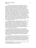
If the price of the product, mousetraps in this example, increases, the employer’s
demand for mousetrap makers will shift—say, from D
1
to D
2
in Figure 15.1. Because the
market value of the laborers’ marginal product has risen, producers now want to sell
more mousetraps and will hire more workers to produce them. Look back again at Table
15.1. If the price of mousetraps rises from $2 to $4, the value of each worker’s marginal
product doubles. At a wage rate of $10 an hour, an employer can now hire as many as
four workers. (Similarly, if the price of the final product falls below $2, the demand for

workers will also fall.)

1
The reader may get the impression that the market demand curve for labor is derived by horizontally
summing the value of marginal product curves of individual firms, which are derived directly from tables
like Table 15.1. Strictly speaking, that is not the case. However, these are refinements of theory that will
be reserved for other, more advanced textbooks and courses.

Chapter 15 Competitive and Monopsonistic
Labor Markets



4

When technological change improves worker productivity, the demand for
workers may increase. If workers produce more, the value of their marginal product may
rise, and employers may then be able to hire more of them. Such is not always the case,
however. Sometimes an increase in worker productivity decreases the demand for labor.
For instance, if worker productivity increases throughout the industry, rather than in just
one or two firms, more mousetraps may be offered on the market, depressing the
equilibrium price. The drop in price reduces the value of the workers’ marginal product
and may outweigh the favorable effect of the increase in productivity. In such cases the
demand for labor will fall. Consumers will pay less, but employees in the mousetrap
industry will have fewer employment opportunities and earn less .

__________________________________
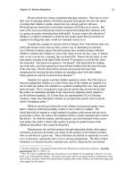
FIGURE 15.1 Shift in Demand for Labor
The demand for labor, like all other demand
curves, slopes downward. An increase in the

demand for labor will cause a rightward shift in the
demand curve, from D
1
to D
2
. A decrease will
cause the leftward shift, to D
3
.





The Supply of Labor
The supply of labor is the assumed positive relationship between the real wage rate and
the number of workers (or work hours) offered for employment during a given period,
everything else held constant. The supply curve for labor generally slopes upward. At
higher wage rates, more workers will be willing to work longer hours than at lower wage
rates (see Figure 15.2). If you survey your MBA classmates, for example, you will
probably find that more of them would be willing to work at a job that paid $50 an hour
than would work for $20 an hour. (At $500 an hour, most would be willing to work
without hesitation, aside for a few lawyers and consultants!)
The supply of labor depends on the opportunity cost of a worker’s time. Workers
can do many different things with their time. They can use it to construct mousetraps, to
do other jobs, to go fishing, and so on. Weighing the opportunity cost of each activity,
the worker will allocate his time so that the marginal benefit of an hour spent doing one
thing will equal the marginal benefit of time that could be used elsewhere. Because some
kinds of work are unpleasant, workers will require a wage to make up for the time lost
from leisure activities like fishing. To earn a given wage, a rational worker will give up

the activities he values least. To allocate even more time to a job (and give up more
valuable leisure-time activities), a worker will require a higher wage.
Chapter 15 Competitive and Monopsonistic
Labor Markets



5

Given this cost-benefit tradeoff, employers who want to increase production have
two options. They can hire additional workers or ask the same workers to work longer
hours. Those who are currently working for $20 an hour must value time spent elsewhere
at less than $20 an hour. To attract other workers, people who value their time spent
elsewhere at more than $20 an hour, employers will have to raise the wage rate, perhaps
to $22 an hour. To convince current workers to put in longer hours – to give up more
attractive alternative activities – employers will also have to raise wage rates. In either
case, the labor supply curve slopes upward. More labor is supplied at higher wages.

____________________________________
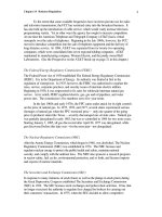
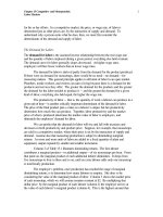
Figure 15.2 Shift in the Supply of Labor
The supply curve for labor slopes upward. An
increase in the supply of labor will cause a rightward
shift in the supply curve from S
1
to S
2
. A decrease in
the supply of labor will cause a leftward shift in the
supply curve, from S
1

to S
3
.
____________________________________





The supply curve for labor will shift if the value of employees’ alternatives
changes. For example, if the wage that mousetrap makers can earn in toy production
goes up, the value of their time will increase. The supply of labor to the mousetrap
industry should then decrease, shifting upward and to the left from S
1
to S
3
, in Figure
15.2. This shift in the labor supply curve means that less labor will be offered at any
given wage rate, in a particular labor market. To hire the same quantity of labor—to keep
mousetrap makers from going over to the toy industry—the employer must increase the
wage rate.
The same general effect will occur if workers’ valuation of their leisure time
changes. Because most people attach a high value to time spent with their families on
holidays, employers who want to maintain operations then generally have to pay a
premium for workers’ time. The supply curve for labor on holidays lies above and to the
left of the regular supply curve. Conversely, if for any reason the value of workers’
alternatives decreases, the supply curve for labor will shift down to the right. If wages in
the toy industry fall, for instance, more workers will want to move into the mousetrap
business, increasing the labor supply in the mousetrap market.

Chapter 15 Competitive and Monopsonistic
Labor Markets



6

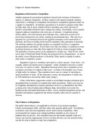
Equilibrium in the Labor Market
A competitive market is one in which neither the individual employer nor the individual
employee has the power to influence the wage rate. Such a market is shown in Figure
15.3. Given the supply curve S and the demand curve D, the wage rate will settle at W
1
,
and the quantity of labor employed will be Q
2
. At that combination, defined by the
intersection of the supply and demand curves, those who are willing to work for wage W
1

can find jobs.
The equilibrium wage rate is determined much as the prices of goods and services
are established. At a wage rate of W
2
, the quantity of labor employers will hire is Q
1
,
whereas the quantity of workers willing to work is Q
3
. In other words, at that wage rate a

surplus of labor exists. Note that all the workers in this surplus except the last one are
willing to work for less than W
2
. That is, up to Q
3
, the supply curve lies below W
2
. The
opportunity cost of these workers’ time is less than W
2
. They can be expected to accept a
lower wage, and over time they will begin to offer to work for less than W
2
. Other
unemployed and employed workers must then compete by accepting still lower wages.
In this manner the wage rate will fall toward W
1
. In the process, the quantity of labor that
employers can afford to hire will expand from Q
1
toward Q
2
.

___________________________________
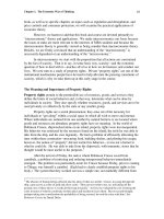
FIGURE 15.3 Equilibrium in the Labor Market
Given the supply and demand curves for labor S and
D, the equilibrium wage will be W
1
, and the

equilibrium quantity of labor hired, Q
2
. If the wage
rate rises to W
2
, a surplus of labor will develop,
equal to the difference between Q
3
and Q
1
.




Meanwhile, the falling wage rate will convince some workers to take another
opportunity, such as going fishing or getting another job. As they withdraw from the
market, the quantity of labor supplied will decline from Q
3
toward Q
2
. The quantity
supplied will meet the quantity demanded—and eliminate the surplus—at a wage rate of
W
1
.
In practice, the money wage rate—the number of dollars earned per hour—may
not fall. Instead, the general price level may increase while the money wage rate remains
constant. But the real wage rate—that is, what the money wage rate will buy—still falls,
producing the same general effects: fewer laborers willing to work, and more workers

demanded by employers. When economists talk about wage increases or decreases, they
mean changes in the real wage rate, or in the purchasing power of a worker’s paycheck.
Chapter 15 Competitive and Monopsonistic
Labor Markets



7

Conversely, if the wage rate falls below W
1
, the quantity of labor demanded by
employers will exceed the quantity supplied, creating a shortage. Employers, eager to
hire more workers at the new cheap wage, will compete for the scarce labor by offering
slightly higher wages. The quantity of labor offered on the market will increase, but at
the same time these slightly higher wages will cause some employers to cut back on their
hiring. In short, in a competitive market, the wage rate will rise toward W
1
, the
equilibrium wage rate.

Why Wage Rates Differ
In a world of identical workers doing equivalent jobs under conditions of perfect
competition, everyone would earn the same wage. In the real world, of course, workers
differ, jobs differ, and various institutional factors reduce the competitiveness of labor
markets. Some workers therefore earn higher wages than others. Indeed, the differences
in wages can be inordinately large. (Compare the hourly earnings of Sylvester Stallone
to those of elementary school teachers.) Wages differ for many reasons, including
differences in the nonmonetary benefits (or costs) of different jobs. Conditions in
different labor markets may differ in such a way as to cause wages to differ. Differences

in the inherent abilities and acquired skills of workers can generate substantial differences
in wages. Finally, discrimination against various groups often lowers the wages of
people in those groups.

Differences in Nonmonetary Benefits
So far we have been speaking as if the wage rate were the key determination of
employment. What about job satisfaction and the way employers treat their employees—
are these issues not important? Some people accept lower wages in order to live in the
Appalachians or the Rockies: college professors forgo more lucrative work to be able to
teach, write, and set their own work schedules. The congeniality of their colleagues is
another significant nonmonetary benefit that influences where and how much people
work. Power, status, and public attention also figure in career decisions.
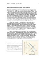
The tradeoffs between the monetary and nonmonetary rewards of work will affect
the wage rates for specific jobs. The more importance people place on the nonmonetary
benefits of a given job, the greater the labor supply. Added to wages, nonmonetary
benefits could shift the labor supply curve from S
1
to S
2
in Figure 15.4, lowering the wage
rate from W
2
to W
1
. Even though the money wage rate is lower, however, workers are
better off according to their own values. At a wage rate of W
1
, their nonmonetary
benefits equal the vertical distance between points a and b, making their full wage equal
to W

3
. The full wage rate is the sum of the money wage rate and the monetary
equivalent of the nonmonetary benefits of a job.
Workers who complain they are paid less than workers in other occupations often
fail to consider their full wages (money wage plus nonmonetary benefits). The worker
with a lower monetary wage may be receiving more nonmonetary rewards, including
Chapter 15 Competitive and Monopsonistic
Labor Markets



8

freedom from intense pressure, comfortable surroundings, and so on. The worker with
the higher money wage may actually be earning a lower full wage than the worker with
nonmonetary income. Certainly many executives must wonder whether their high
salaries compensate them for their lost home life and leisure time, and teachers who envy
the higher salaries of coaches should recognize that a somewhat higher wage rate is
necessary to offset the increased risk of being fired that goes with coaching.
Employers can benefit from providing employees with nonwage benefits. A
favorable working climate attracts more workers at lower wages. Although benefits can
be costly, they are worthwhile as long as they lower wages more than they raise other
labor costs. Some nonwage benefits, like air conditioning and low noise levels, also raise
worker productivity. Needless to say, an employer cannot justify unlimited nonwage
benefits. Employers will not pay more in wages, monetary or nonmonetary, than a
worker is worth. In a competitive labor market they will tend to pay all employees a
wage rate equal to the marginal value of the last employee hired.

_________________________________________
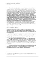
FIGURE 15.4 The Effect of Nonmonetary

Rewards on Wage Rates
The supply of labor is greater for jobs offering non-
monetary benefits—S
2
rather than S
1
. Given a
constant demand for labor, the wage rate will be
W
2
for workers who do not receive nonmonetary
benefits and W
1
for workers who do. Even though
wages are lower when nonmonetary benefits are
offered, workers are still better off; they earn a
total wage equal, according to their own values, to
W
3
.



Differences Among Markets
Differences in nonmonetary benefits explain only part of the observed differences in
wage rates. Supply and demand conditions may differ between labor markets. As Figure
15.5 shows, given a constant supply of labor, S, a greater demand for labor will mean a
higher wage rate. Conversely, given a constant demand for labor will mean a lower wage
rate. Depending on the relative conditions in different markets, wages may—or may
not—differ significantly.

People in different lines of work may also earn different wages because
consumers value the products they produce differently. Automobile workers may earn
more than textile workers because people are willing to pay more for automobiles than
for clothing. Consumer preferences contribute to differences in the value of the marginal
product of labor and ultimately in the demand for labor.
Chapter 15 Competitive and Monopsonistic
Labor Markets



9

By themselves, relative product values cannot explain long-run differences in
wages. Unless textile work offers compensating nonmonetary benefits, laborers in that
industry will be attracted to higher wages elsewhere, perhaps in the automobile industry.
The supply of labor in the automobile industry will rise, and the wage rate will fall. In
the long run, the wage differential will decrease or even disappear.
Certain factors may perpetuate the money wage differential in spite of
competitive market pressures. Textile workers who enjoy living in North or South
Carolina may resist moving to Detroit, Michigan, where automobiles are manufactured.
In that case, the nonmonetary benefits associated with textile work offset the difference in
money wages. In addition, the cost of acquiring the skills needed for automobile work
may act as a barrier to movement between industries—a problem we will address shortly.

FIGURE 15.5 The Effect of Differences in Supply and Demand on Wage Rates
In competitive labor markets, higher demand for labor (D
2
in part (a)) will bring a higher wage rate. A
higher supply of labor (S2 in part (b)) will bring a lower rate

Differences Among Workers
Differences in labor markets do not explain wage differences among people in the same
line of work. Differences among workers must be responsible for that disparity. Some
people are more attractive to employers. Employers must pay such workers more
because their services are eagerly sought after, but they can afford to pay them more,
because their marginal product is greater.
Mark McGuire earns an extremely high salary. The St. Louis Cardinals are
willing to pay him so well both because of his popularity among fans when McGuire
Chapter 15 Competitive and Monopsonistic
Labor Markets



10

plays, ballpark crowds are bigger—and because he is a successful hitter. Because a

winning team generally attracts more support than a losing one. McGuire’s presence
indirectly boosts the team’s earnings. In other words, McGuire is in a labor submarket
like the one shown by curve D
2
in Figure 15.5(a). Other players are in submarket D
1
.
Differences in skill may also account for differences in wages. Most wages are
paid not just for a worker’s effort but also for the use of what economists call human
capital. Human capital is the acquired skills and productive capacity of workers. We
usually think of capital as plant and equipment—for instance, a factory building and the
machines it contains. A capital good is most fundamentally defined, however, as
something produced or developed for use in the production of something else. In this
sense capital goods include the education or skill a person acquires for use in the
production process. The educated worker, whether a top-notch mechanic or a registered
nurse, holds within herself capital assets that earn a specific rate of return. In pursuing
professional skills, the worker, much like the business entrepreneur, takes the risk that the
acquired assets will become outmoded before they are fully used. In the 1970’s and
1980’s students who majored in history expecting to teach found that their investment in
human capital did not pay off. Many were unable to get jobs in their chosen field.
Finally, wage differences can result from social discrimination, whether sexual,
racial, religious, ethnic, or political. Potential employees are often grouped according to
some easily identifiable characteristic, such as sex or skin color. Employment decisions
are then made primarily on the basis of the group to which the individual belongs, rather
than on individual merit. Thus a qualified woman may not be considered for an
executive job because women as a group are excluded. To the extent that employers
prefer to work with certain groups, like whites or men, the labor market will be
segmented. Employees in different submarkets, with different demand curves and wage
differentials, will be unable to move easily from one market to another. The barriers to
the free movement of workers allow wage differences to persist.

Competition among producers in the market for final goods can weaken (but not
necessarily eliminate) discriminatory practices. Suppose employers harbor a deep-seated
prejudice against women, which depresses the market demand and wage rates for female
workers. If there is no rational reason for preferring men—if women are just as
productive as men—an enterprising producer can hire women, pay them less, undersell
the other suppliers, and take away part of their markets. Under competitive pressure,
employers will start to hire women in order to keep their market shares. As a result, the
demand for women workers will rise, while the demand for men will fall. Such
competition may not eliminate the wage differential between men and women, but it can
reduce it. In industries where employers exercise market power, social discrimination
may persist.

Stricter Housing Standards for Migrants
In the 1960s, television news documentaries have publicized the substandard, even
squalid housing commonly provided to migrant farm workers. Most housing for
Chapter 15 Competitive and Monopsonistic
Labor Markets



11

migrants lacked plumbing and running water. Sleeping arrangements consisted of a few
mattresses thrown on the floor.
To many, the obvious solution to the problem was to impose stricter housing
standards on employers of migrant workers. Yet one consequence of such legislation had
been reduced employment opportunities for migrant workers.
2

Figure 15.6 shows how
the increased nonmonetary benefits lowered the demand for migrant labor. In a
completely free market, employers are willing to pay a money wage of W
2
for migrant
labor. If they are forced to pay workers more by meeting higher housing standards, their
demand curve for migrant labor will fall from D
1
to D
2
. The equilibrium money wage
rate will fall to W
1
, and employment opportunities will be reduced from Q
3
to Q
2
. Again,
as in the case of the minimum wage, those who keep their jobs may be better off. Their
full wage rate will rise from W
2
to W
3
(W
1
in money wages plus W
3
– W
1
in nonmonetary

benefits), but the workers who are not hired will suffer a loss in income.

_________________________________________
FIGURE 15.6 The Effect of Stricter Housing
Standards on Employment
Higher housing standards for migrant workers will
reduce employers’ demand for migrant labor from
D
1
to D
2
. The money wage rate will fall from W
2

to W
1
, but the nonmonetary benefits of improved
housing will increase by the vertical distance
between points a and b. Although workers will be
earning a full wage of W
3
, fewer of them—Q
2

instead of Q
3
—will be hire

2
Milton Friedman, “Migrant Workers,” Newsweek (July 27, 1970): 60.

Chapter 15 Competitive and Monopsonistic
Labor Markets





The farmers who employ migrant workers are caught in a competitive bind.
Consumers want to buy their food at the lowest possible price. As producers, farmers
must be able to sell their produce at a competitive price. That means minimizing the cost
of production, including the full wage rate paid to employees. If farmers are forced to
provide better housing for their laborers, they must reduce costs in other ways, including
the substitution of machinery for labor. This is precisely what happened in many farm
areas since the imposition of stricter housing standards. A federal law establishing
migrant housing standards was passed in the late 1960s. In 1969 the farm labor service
of the Michigan Employment Security Commission arranged jobs and housing for 27,163
migrants, but in the summer of 1970 it estimated that it would be able to place only 7,000
to 8,000 workers. State and local officials forecast that on balance, the new housing
standards would eliminate 6,000 to 10,000 jobs. Meanwhile many growers, stung by the
bad publicity surrounding migrant housing, closed their camps and switched to
mechanical harvesting. As one grower put it, “It might be cheaper for me to continue
using migrant help for a few more years, but mechanization is the trend of the future.
And no matter what kind of housing I provide I’m going to be criticized for mistreating
migrants. So I might as well switch now.”
3



Monopsonistic Labor Markets

Competition is bad for those who have to compete. Not only as producers but as
employers, firms would rather control competitive forces than be controlled by them.
They would like to pay employees less than the market wage—but competition does not
give them that choice
Similarly, workers find that competition for jobs prevents them from earning more
than the market wage. Thus doctors, truck drivers, and barbers have an interest in
restricting competition in their labor markets. Acting as a group, they can acquire some
control over their employment opportunities and wages.
Such power is difficult to maintain without the support of the law or the threat of
violence, whether real or imagined. It comes at the expense of the consumer, who will
have fewer goods and services to choose from at higher prices. As always, the exercise
of power by one group leads not only to market inefficiencies but also to attempts by
other groups to counteract it. The end result can be reduction in the general welfare of
the community.
This section examines both employer and employee power in the labor market; the
conditions that allow it to persist; its influence on the allocation of resources; and its
effects on the real incomes of workers, consumers, and entrepreneurs.



3
“Housing Dispute Spurs Migrant Farmers to Switch to Machines from Migrant Help,” Wall Street
Journal, June 29, 1970, p. 18
Chapter 15 Competitive and Monopsonistic
Labor Markets




13

The Monopsonistic Employer
Power is never complete. It is always circumscribed by limitations of knowledge and the
forces of law, custom, and the market. Within limits, employers can hire and fire, and
can decide what products to produce and what type of labor to employ. Laws restrict the
conditions of employment (working hours, working environment) they may offer,
however, as well as their ability to discriminate among employees on the basis of sex,
race, age, or religious affiliation. Competition imposes additional constraints. In a
highly competitive labor market, an employer who offers very low wages will be outbid
by others who want to hire workers. Competition for labor pushes wages up to a certain
level, forcing some employers to withdraw from the market but permitting others to hire
at the going wage rate.
4

For the individual employer, then, the freedom of the competitive market is a highly
constrained freedom. Not so, however, for those lucky employers who enjoy the power
of a monopsony. A pure monopsony is the sole buyer of a good, service, or resource.
(Monopsony should not be confused with monopoly, the single seller of a good and
service.) The term is most frequently used to indicate the sole or dominant employer of
labor in a given market. A good example of a monopsony would be a large coal-mining
company in a small town with no other industry. A firm that is not a sole employer but
that dominates the market for a certain type of labor is said to have monopsony power.
Monopsony power is the ability of a producer to alter the price of a resource by
changing the quantity employed. By reducing competition for workers’ services,
monopsony power allows employers to suppress the wage rate.

_________________________________________
FIGURE 15.7 The Competitive Labor Market
In a competitive market, the equilibrium wage rate
will be W

2
. Lower wage rates, such as W
1
, would
create a shortage of labor, and employers would
compete for the available laborers by offering a
higher wage. In pushing up the wage rate to the
equilibrium level, employers impose costs on one
another. They must pay higher wages not only to
new employees, but also to all current employees,
in order to keep them.






4
Competitors who do not hire influence the wage rate just as much as those who do; their presence on the
sidelines keeps the price from falling. If firm lowers its wages, other employers may move into the market
and hire away part of the work force.
Chapter 15 Competitive and Monopsonistic
Labor Markets




14

The Cost of Labor

Monopsony power reduces the costs of competitive hiring. Assume that the downward-
sloping demand curve D in Figure 15.7 shows the market demand for workers, and the
upward-sloping supply curve S shows the number of workers willing to work at various
wage rates. If all firms act independently—that is, if they compete with one another—the
market wage rate will settle at W
2
, and the number of workers hired will be Q
2
. At lower
wage rates, such as W
1
, shortages will develop. As indicated by the market demand
curve, employers will be willing to pay more than W
1
. If a shortage exists, the market
wage will be bid up to W
2
.
An increase in the wage rate will encourage more workers to seek jobs. As long as
there is a shortage, however, the competitive bidding imposes costs on employers. The
firm that offers a wage higher than W
1
forces other firms to offer a comparable wage to
retain their current employees. If those firms want to acquire additional workers, they
may have to offer an even higher wage. As they bid the wage up, firms impose
reciprocal costs on one another, as at an auction.
Because any increase in wages paid to one worker must be extended to all, the total
cost to all employers of hiring even one worker at a higher wage can be staggering. If the
wage rises from W
1

to W
2
in Figure 15.7, the total wage bill for the first Q
1
workers rises
by the wage increase W
2
– W
1
times Q
1
workers. Table 15.2 shows how the effect of a
wage increase is multiplied when it must be extended to other workers. The first two
columns reflect the assumption that as the wage rate rises, more workers will accept jobs.
If only one worker is demanded, he can be hired for $20,000. The firm’s total wage bill
will also be $20,000 (column 3). If two workers are demanded, and the second worker
will not work for less than $22,000, the salary of the first worker must also be raised to
$22,000. The cost of the second worker is therefore $24,000 (column 4): $22,000 for his
services plus the $2,000 raise that must be given to the first worker.


TABLE 15.2 Market Demand for Tomatoes

Number of
Workers Willing
to Work
(1)
Annual Wage
of Each
Worker

(2)
Total Wage
Bill
[(1) times (2)]
(3)
Marginal Cost of
Additional Worker
[Change in (3)]
(4)
1
2
3
4
5
6
$20,000
22,000
24,000
26,000
28,000
30,000
$ 20,000
44,000
72,000
104,000
140,000
180,000
$20,000
24,000
28,000

32,000
36,000
40,000

Chapter 15 Competitive and Monopsonistic
Labor Markets




15

The cost of additional workers can be similarly derived. When the sixth worker is
added, she must be offered $30,000 and the other five workers must each be given a
$2,000 raise. The cost of adding this new worker, called the marginal cost of labor, has
risen to $40,000. The marginal cost of labor is the additional cost to the firm of
expanding employment by one additional worker. Note that as the number of workers
hired increases, the gap between the marginal cost of labor and the going wage rate
expands. When two workers are hired, the gap is $2,000 ($24,000-$22,000). When six
are employed, it is $10,000 ($40,000-$30,000).
Figure 15.8, based on columns 1 and 4 of Table 15.2, shows the marginal cost of
labor graphically. The marginal cost curve lies above the supply curve, for the cost of
each new worker hired (beyond the first worker) is greater than the worker’s salary.


_________________________________________
FIGURE 15.8 The Marginal Cost of Labor
The marginal cost of hiring additional workers is
greater than the wages that must be paid to the new
workers. Therefore the marginal cost of labor

curve lies above the labor supply curve








The Monopsonistic Hiring Decision
The monopsonistic employer does not get caught in the competitive bind. By definition
it is the only or dominant employer. Like a monopolist, the monopsonist can search
through the various wage-quantity combinations on the labor supply curve for the one
that maximizes profits. The monopsonist will keep hiring more workers as long as their
contribution to revenues is greater than their additional cost, as shown by the marginal
cost of labor curve MC in Figure 15.9. To maximize profits, in other words, the
monopsonist will hire until the marginal cost of the last worker hired (MC) equals his
marginal value, as shown by the textiles market demand curve for labor. Given the
demand for labor D, the monopsonist’s optimal employment level will be Q
2
, where the
marginal cost and demand for labor curves intersect. Note that that level is lower than
the competitive employment level, Q
3
.
Chapter 15 Competitive and Monopsonistic
Labor Markets

16

Why hire where marginal cost equals marginal value? Suppose the monopsonist
employed fewer workers—say Q
1
. The marginal value of worker Q
1
would be quite high
(point a), while her marginal cost would be low (point b). The monopsonist would be
forgoing profits by hiring only Q
1
workers. Beyond Q
2
workers, the reverse would be
true. The marginal cost of each new worker would be greater than his marginal value.
Hiring more than Q
2
workers would reduce profits.
Once the monopsonist has chosen the employment level Q
2
, it pays workers no
more than is required by the labor supply curve, S. In Figure 15.9, the monopsonist must
pay only W
1
—much less than the wage that would be paid in a competitive labor market,
W
2
. In other words, the monopsonist hires fewer workers and pays them less than an
employer in a competitive labor market.

_________________________________________
FIGURE 15.9 The Monopsonist
The monopsonist will hire up to the point where
the marginal value of the last worker, shown by the
demand curve for labor, equals his or her marginal
cost. For this monopsonistic employer, the
optimum number of workers is Q
2
. The
monopsonist must pay only W
1
for that number of
workers—less than the competitive wage level, W
2
.






It is the monopsonistic firm’s power to reduce the number of workers hired that
enables it to hold wages below the competitive level. In a competitive labor market, if
one firm attempts to cut employment and reduce wages, it will not be able to keep its
business going, for workers will depart to other employers willing to pay the going
market wage. The individual firm is not large enough in relation to the entire labor
market to exercise monopsony power. It therefore must reluctantly accept the market
wage, W

2
, as a given.

Employer Cartels: Monopsony
Power through Collusion
Envying the power of the monopsonist, competitive employers may attempt to organize a
cartel. A employer cartel is any organization of employers that seeks to restrict the
number of workers hired in order to lower wages and increase profits.
Chapter 15 Competitive and Monopsonistic
Labor Markets




17

The usual way of lowering employment is to establish restrictive employment rules
that limit the movement of workers from one job to another. Such rules tend to reduce
the demand for labor. In Figure 15.10, demand falls from D
1
to D
2
. As a result, the wage
rate drops, from W
2
to W
1
, and employment falls, from Q
3
to Q

2
. Although the method of
limiting employment is different from that used in monopsony, the effect is the same.
Whether the monopsonistic firm equates marginal cost with marginal value (shown by
curve D
1
) or the employer cartel reduces the demand for labor (to D
2
), employment still
drops to Q
2
. In both cases workers earn a wage rate of W
1
—less than the competitive
wage.
One industry in which employers have tried to cartelize the labor market is
professional sports. Owners of teams have developed complex rules governing the hiring
of athletes. In the National Football League (NFL), for example, teams acquire rights to
negotiate with promising college players through an annual draft. Once one team has
drafted a player, no other team in the league can negotiate with him (unless he remains
unsigned until the next year’s draft). Teams can buy and sell draft rights as well as rights
to players already drafted, but within leagues they are prohibited from competing directly
with one another for players’ services. Violations of these rules carry stiff penalties,
including revocation of a team’s franchise.


__________________________________________
FIGURE 15.10 The Employer Cartel
To achieve the same results as a monopsonist, the
employer cartel will devise restrictive employment

rules that artificially reduce market demand to D
2
.
The reduced demand allows cartel members to hire
only Q
2
workers at wage W
1
—significantly less than
the competitive wage, W
2
.
___________________________________






MANAGER’S CORNER I: Paying for Performance
To this point in the chapter, our discussion has been focused on how labor “markets”
work, and our interest has been on how the wage rate and other benefits are determined
by the broad forces of supply and demand. However, markets must ultimately work with
the interests of workers in mind. The problem most firms must solve is how to get
Chapter 15 Competitive and Monopsonistic
Labor Markets

18

workers to do what they are supposed to do, which is work effectively and efficiently
together for the creation of firm profits. This is no mean task, as we will see at various
points in this book. There is a lot of trial and error in business, especially as it relates to
how workers are paid. At the same time, thinking conceptually about the
payment/incentive problem can help firms moderate the extent of errors in business.
One of the most fundamental rules of economics, and the reason d’être the
discussions in the “Manager’s Corners,” is that if you offer people a greater reward, then
they will do more of whatever is being rewarded, everything else equal. Many people
find this proposition to be objectionable, because it implies that people can, to one degree
or another, be “bought.” Admittedly, incentives may not matter in all forms of behavior;
some people will sacrifice their lives rather than forsake a strongly held principle.
However, the proposition that incentives matter does seem to be applicable to a
sufficiently wide range of behavior to be considered a “rule” that managers are well
advised to keep in mind: Pay someone a higher wage such as time and a half and
they will work overtime. Pay them double time, and they will even work holidays.
There is some rate of pay at which a lot of people will work almost any time of the day or
night on any day of the year.
This rule for incentives is not applicable only to the workplace. Parents know that
one of the best ways to get their children to take out the garbage is to tie their allowance
to that chore. Moreover, patients in psychiatric hospitals, many of whom have literally
lost virtually all capacity for rational discourse, appear to respond to incentives.
According to research, if mentally ill, institutionalized patients are paid for the simple
tasks they are assigned (for example, sweeping a room or picking up trash), they will
perform them with greater regularity.
5

Even pigeons, well known for having the lowest form of birdbrains, respond to
incentives. Granted, pigeons may never be able to grasp the concept of monetary rewards

(offering them a dollar won’t enlist much of a response), but pigeons apparently know
how to respond to food rewards (offer a nut in the palm of your outstretched hand and a
whole flock will descend, and maybe leave their mark, on your shoulder). From research,
we also know that pigeons are willing to work measured by how many times they peck
colored levers in their cages to get food pellets, and they will work harder if the reward
for pecking is raised. Researchers have also been able to get pigeons to loaf on the job
just like humans. How? Simply lower their rate of “pay.”
6


The “Right” Pay
It would appear that rules of incentives would lead managers everywhere to make sure
that workers have the right incentives by always tying pay to some measure of
performance. Clearly, the lone worker in a single proprietorship has the “right”
incentive. His or her reward is the same as the reward for the whole firm. The full cost

5
See Richard B. McKenzie and Gordon Tullock, The New World of Economics (New York: McGraw-Hill,
1994), chap. 4.
6
Ibid.
Chapter 15 Competitive and Monopsonistic
Labor Markets




19

of any shirking is borne by the worker/owner. However, such a congruence between the

rewards of the owners and workers is nowhere else duplicated. There are always “gaps”
between the goals of the owners and the workers, and the greater the number of workers,
typically, the greater the gap in incentives. In very large firms, workers have greatly
impaired incentives to pursue the goals of the owners. The workers are far removed from
the owners by layers of bureaucracy, communications on firm goals are often imperfect,
and each worker at the bottom of the firm pyramid can reason that his or her
contributions to firm revenues and goals, or the lack of them, can easily go undetected. A
reoccurring theme of this book is that when monitoring is difficult, one can expect many
workers to exploit opportunities at their disposal.
And the opportunities taken can result in substantial losses in worker output.
Management specialist Edward Lawler reported that during a strike at a manufacturing
firm, a secretary was asked to take over a factory job and was paid on a piece rate basis.
Despite no previous experience, within days she was turning out 375 percent more output
than the normal worker who had spent 10 years on the job and was constantly
complaining that the work standards were too demanding.
7
Obviously, the striking
workers had been doing something other than working on the job.
How can managers improve incentives, reduce shirking, and increase worker
productivity? At the turn of the century, the great management guru Frederick Taylor
strongly recommended piece-rate pay as a means of partially solving what he termed the
“labor problem,” but he was largely ignored in his own time by both management and
labor, and for the good reasons discussed in this chapter.
8

There is a multitude of ways of getting workers to perform that don’t involve
money pay, and many of the ways are studied in disciplines like organizational behavior,
which draws on the principles of psychology. Managers do need to think about patting
workers on the back once in a while, clearly defining corporate goals, communicating
goals in a clear and forceful manner, and exerting leadership.

Southwest Airlines, one of the more aggressive, cost-conscious, and profitable
airlines, motivates its workers by creating what one analyst called a “community . . .
resembling a 17th century New England town more than a 20th century corporation.” The
airline bonds its workers with such shared values as integrity, trust, and altruism.
9
But, a
company with a productive corporate culture is almost surely a company with strong
incentives in place to reward productivity. Without taking anything away from the
corporate culture at Southwest Airlines, it should, however, be pointed out that one
reason it has the lowest cost in the business is that its pilots and flight attendants are paid
by the trip. This, along with a strong corporate culture, explains why Southwest's pilots
and flight attendants hustle when the planes are on the ground. Indeed, Southwest has the
shortest turn-around time in the industry. It pays the crews to do what they can to get

7
Edward E. Lawler, III, Strategic Pay: Aligning Organizational Strategies and Pay Systems (San Francisco:
Jossey-Bass Publishers, 1990), p. 58.
8
Frederick W. Taylor, “A Piece Rate System,” American Society of Mechanical Engineers Transactions,
vol. 16 (1895), pp. 856-893.
9
William G. Lee, “The New Corporate Republics,” Wall Street Journal (September 26, 1994), p. 12.
Chapter 15 Competitive and Monopsonistic
Labor Markets




20

their planes back in the air.
10
Motorola organizes its workers into teams and allows them
to hire and fire their cohorts, determine training procedures, and set schedules. Federal
Express’ corporate culture includes giving workers the right to evaluate their bosses and
to appeal their own evaluations all the way to the chairman. But, still, it’s understandable
why Federal Express delivery people move at least twice as fast as U.S. postal workers:
FedEx workers have incentives to do so, whereas postal workers do not.
11

We don’t want to criticize the traditional, non-incentive methods for getting
things done in business. Indeed, we have taken up the issue of “teams” discussed much
earlier in the book, and the importance of virtues like “trust” will be raised before we
conclude this chapter. At the same time, we wish to stress a fairly general and
straightforward rule for organizing much production: Give workers a direct detectable
stake in firm revenues or profits in order to raise revenues and profits. Pay for
performance. One means of doing that is to make workers’ pay conditional on their
output: the greater the output from each worker, the greater the individual worker’s pay.
Ideally, we should dispense with salaries, which are paid by the week or year, and
always pay by the “piece” or “piece rate.” Many firms for example, hosiery mills
do pay piece rate; they pay by the number of socks completed (or even the number of
toes closed). Piece rate can be expected to raise wages of covered workers for two
reasons: First, the incentives can be expected to induce workers to work harder for more
minutes of each hour and for more hours during the workday. Second, the piece-rate
workers will be asked to assume some of the risk of production, which is influenced by
factors beyond the workers’ control. For example, how much each worker produces will
be determined by what the employer does to provide workers with a productive work
environment and what other workers are willing to do. So, piece-rate workers can be
expected to demand and receive a risk premium in their paychecks. One study has, in
fact, shown that a significant majority of workers covered under “output-related

contracts” in the nonferrous foundries industry earn between 5 percent and 12 percent,
depending on the occupation, more than their counterparts who are paid strictly by their
time at work. Of that pay differential, about a fifth has been attributable to risk bearing
by workers, which means that a substantial share of the pay advantage for incentive
workers is attributable to the greater effort expended by the covered workers.
12

However, such a rule – paying by the piece is hardly universally adopted.
Indeed, piece-rate workers probably make up a minor portion of the total work force (we
have not been able to precisely determine how prevalent piece-pay systems are). Many
automobile salespeople, of course, are paid by the number of cars sold. Many lawyers
are paid by the number of hours billed (and presumably services provided). Musicians
are often paid by the number of concerts played.

10
Howard Banks, "A Sixties Industry in a Nineties Economy," Forbes, May 9, 1994: pp. 107-112.
11
FedEx actually tracks its delivery people on their routes, and the workers understand that their pay is tied
to how cost-effective they are in their deliveries. Postal workers understand that they are not being so
carefully monitored, mainly because there are no stockholders who can claim the profits from a speed-up in
their work.
12
Tron Petersen, “Reward Systems and the Distribution of Wages,” Journal of Law, Economics, and
Organizations, vol. 7 (special issue), 1991, pp. 130-158.
Chapter 15 Competitive and Monopsonistic
Labor Markets

21

But there are relatively few workers in manufacturing and service industries
whose pay is directly tied to each item or service produced. Professors are not paid by
the number of students they teach. Office workers are not paid by the number of forms
processed or memos sent. Fast food workers are not paid by the number of burgers
flipped. Most people’s pay is, for the most part, directly and explicitly tied to time on the
job. They are generally paid by the hour or month or even year.
Admittedly, the pay of most workers has some indirect and implicit connection to
production. Many workers know that if they don’t eventually add more to the revenues
of their companies than they take in pay, their jobs will be in considerable jeopardy. The
question we find interesting is why “piece rate” or “pay for performance” is not a
more widely employed pay system, given the positive incentives it potentially provides.
Many explanations for the absence of a piece-rate pay system are obvious and
widely recognized.
13
The output of many workers cannot be reduced to “pieces.” In
such cases, no one should expect pay to be tied to that which cannot be measured with
tolerable objectivity. Our work as university professors is hard to define and measure. In
fact, observers might find it hard to determine when we are working, given that while at
work, we may be doing nothing more than staring at a computer screen or talking with
students in the hallways. Measuring the “pieces” of what secretaries and executives do is
equally, if not more, difficult.
If a measure of “output” is defined when the assigned tasks are complex, the
measure will not likely be all-inclusive. Some dimensions of the assigned tasks will not
be measured, which means that workers’ incentives may be grossly distorted. They may
work only to do those things that are defined and measured and related to pay at the
expense of other parts of their assignments. If workers are paid by the number of parts
produced, with the quality of individual parts not considered, some workers could be
expected to sacrifice quality in order to increase their production count. If professors

were paid by the number of students in their classes, you can bet they would spend less
time at research and in committee meetings (which would not be all bad). If middle
managers were paid solely by units produced, they would produce a lot of units with little
attention to costs. There is an old story from the days before the fall of communism in
the former Soviet Union. According to the story, the managers of a shoe factory were
given production quotas for the number of shoes they had to make, and they were paid
according to how much they exceeded their quota. What did they do? They produced
lots of shoes, but only left ones!
Much work is the product of “teams,” or groups of workers, extending, at times,
to the entire plant or office. Pay is often not related to output because it may be difficult
to determine which individuals are responsible for the “pieces” that are produced.

13
For a review of arguments offered by psychologists against incentive pay plans, see Alfie Kohn, “Why
Incentive Plans Cannot Work,” Harvard Business Review September-October 1993, pp. 54-63. Kohn sums
up his argument, “Do rewards motivate people? Absolutely. They motivate people to get rewards” (p. 62),
suggesting that the goals of the firm might not be achieved in the process, given the complexity of the
production process and the margins workers can exploit. Kohn’s criticisms are reviewed and critiqued in
the last chapter of this book.
Chapter 15 Competitive and Monopsonistic
Labor Markets




22

Because we took up the problems of forming and paying teams in an earlier chapter, we
only remind readers that team production creates special incentive problems. Making the
teams “small” is one way to enhance incentives by making the contributions, or lack

thereof, of each team member noticeable to others on the team.
When workers are paid by salary, they are given some assurance that their
incomes will not vary with firm output, which can go up and down for many reasons, not
under their control. For example, how many socks a worker can stitch at the toe is
dependent upon the flow of socks through the plant, over which the workers who do the
stitching may have no control. When workers are paid by the piece, they are, in effect,
asked to assume a greater risk that shows up in the variability of the income they take
home. Granted, piece rate may give the workers a higher average income. However, in
order for the piece rate system to work and be profitable for the firm the increase in
expected worker productivity would have to exceed the risk premium that risk averse
workers would demand. Piece rate (or any other form of incentive compensation) is not
employed in many firms simply because the risk premium workers demand is greater than
their expected increase in productivity. This is often the case because workers tend to be
risk averse (or reluctant to take chances, or assume the costs associated with an uncertain
and variable income stream).
If paid by the work done, workers would also have to worry about how changes in
the general economy would affect their workloads and production levels. A downturn in
the economy, due to forces that are global in scope, can undermine worker pay when pay
is tied to output. When Du Pont introduced its incentive compensation scheme for its
fibers division in 1988 under which a portion of the workers’ incomes could be lost if
profit goals were not achieved and could be multiplied if profit goals were exceeded – the
managers and employees expected, or were told to expect, substantial income gains.
14

However, when the economy turned sour in 1990, employee morale suffered as profits
fell and workers were threatened with reduced incomes. The incentive program was
cancelled before the announced three-year trial period was up.
15
Du Pont obviously
concluded that it could buy back worker morale and production by not subjecting worker

pay to factors that were beyond worker control. Each individual employee could reason
that there was absolutely nothing he could do about the national economy or, for that
matter, about the work effort expended by the 20,000 other Du Pont workers who were
covered by the incentive program. They could rightfully fear that their incomes were
being put at risk by the free riding of all other workers.
This line of analysis leads to the conclusion that piece-rate (and other forms of
incentive) pay schemes will tend to be used in firms where the risk to workers is
relatively low (relative to the benefits of the improved incentives). This means that they
will tend to be used where production is not highly variable and where, in the absence of
piece-rate pay, workers can easily exploit opportunities to shirk. That is, they will tend to
be used where workers cannot be easily monitored. For example, salespeople who are

14
L. Hayes, “All Eyes on Du Pont’s Incentive Program,” Wall Street Journal, December 5, 1988, p. B1.
15
R. Koening, “Du Pont Plan Linking Pay to Fibers Profit Unravels,” Wall Street Journal, October 25,
1990, p. B1.
Chapter 15 Competitive and Monopsonistic
Labor Markets




23

always on the road (which necessarily means that no one at the home office knows much
about what they do on a daily basis) will tend to be paid, at least in part, by the “piece,”
in some form or another, say, by the sale.
Piece-rate pay systems may also be avoided because employers are likely to be in
a better position to assume the risk of production variability than their employees are.

This is because much of the variability in the output of individual workers will be
“smoothed out” within a whole group of employees. When one worker’s output is down,
then another worker’s output will be up. Workers will, in effect, be able to buy
themselves out of the risk. If each of the workers sees the risk cost of the piece-rate
system at $500 and the employer sees the risk cost at $100, then each worker can agree to
give up, say, $110 in pay for the rights to a constant income. The worker gains, on
balance, $390 in non-money income ($500 in risk cost reduction minus the $110
reduction in money wages). The employer gives up the piece-rate system simply because
he or she can make a profit $10 in this example off each worker ($110 reduction in
worker money wages minus the $100 increase in risk cost). One would therefore expect,
other things equal, piece-rate pay schemes would be more prevalent in “small” firms
than in “large” ones. Large employers are more likely to be able to smooth out the
variability.
Also, piece-rate pay systems can only be used when and where employers can
make credible commitments to their workers to abide by the pay system that they
establish and not to cut the rate in the piece-rate when the desired results are achieved.
Unfortunately, all too often managers are unable to make the credible commitment for the
same reason that they might find, in theory, the piece-rate system to be an attractive way
(in terms of worker productivity and firm profits) to pay workers. The basic problem is
that both workers and managers have incentives to engage in opportunistic behavior to
the detriment of the other group.
Managers understand that many workers have a natural inclination to shirk their
responsibilities, to loaf on the job and misuse and abuse company resources with the
intent of padding their own pockets. Managers also know that if they tie their workers’
pay to output, then output may be expected to expand. Fewer workers will exploit their
positions and loaf on the job. At the same time, the workers can reason that incentives
also matter to managers. Like workers, managers are not always angels (and are
sometimes outright devils, just like their workers) and can be expected, to one degree or
another, to exploit their positions, achieving greater personal and firm gains at the
expense of their workers.

Hence, workers can reason that if they respond to the incentives built into the
piece-rate system and produce more for more pay, then managers can change the deal.
The managers can simply raise the number of pieces that the workers must produce in
order to get the previously established pay, or managers can simply dump what will then
be excess workers.
To clarify this point, suppose a worker is initially paid $500 a week, and during
the course of the typical week, he or she produces 100 pieces for an average pay of $5
per piece. Management figures that the worker is spending some time goofing off on the
Chapter 15 Competitive and Monopsonistic
Labor Markets




24

job and that the worker’s output can be raised if he or she is paid $5 for each piece
produced.
If the worker responds by increasing his output to 150 pieces, the management
can simply lower the rate to $3.50 per piece, which would give the worker $525 a week
and would mean that the firm would take the overwhelming share of the gains from the
worker’s not management’s greater efforts. The worker would, in effect, be working
harder and more diligently with little to show for what he or she has done. By heeding
the piece-rate incentive, the worker could be inadvertently establishing a higher
production standard.
These threats are real. Managers at a General Motors panel stamping plant in
Flint, Michigan announced that the company would allow workers to leave after they had
satisfied daily production targets. Workers were soon leaving by noon. Management
responded by increasing production targets. The result was a bitter workforce.
16

So, one reason piece-rate systems aren’t more widely used is that the systems can
be abused by managers, which means that workers will not buy into them at reasonable
rates of pay.
Another way of explaining the lack of use of piece-rate pay is that they often
don’t work as might be expected. Incentives still matter. The problem is that the much
talked-about incentives are not there, or workers don’t believe they are there. And
workers don’t believe the incentives are present because they don’t or can’t believe
that their managers will resist the temptation to gain at their the workers’ expense.
Managers are unable to make what we have, in other contexts, called a credible
commitment (or a position on which workers can rely), meaning they have not been able
to convince their workers that they will not take advantage of them (just as the workers
may have been taking advantage of their managers).
Indeed, the piece-rate system can have the exact opposite effect of the one
intended. We have noted that workers can reason that their managers will increase the
output demands if they produce more for any given rate. However, the implied
relationship between output and production demands should also be expected to run the
other way: That is, the workers can reason that if managers will raise the production
requirements when they produce more in response to any established rate, then managers
should be willing to lower the production requirements when the workers lower their
production after the piece-rate system is established. Hence, the establishment of the
piece-rate system can lead to a reduction in output as workers cut back on production.
The purpose of the incentive pay may be to increase production, but the result can be to
induce lower production standards for the same rate of pay. The workers’ expectation
can be that the rate of pay will be raised.
How? Suppose that the worker responds to the rate of $5 per piece by actually
cutting back his or her total production from 100 to 75 pieces per week. Then
management might be expected to increase the rate to, say, $6.50 per piece, leaving the

16

See Benjamin Klein, Robert Crawford, and Armen Alchian, “Vertical Integration, Appropriable Rents,
and the Competitive Contracting Process,” Journal of Law and Economics, vol. 21 (1978), pp. 297-326.
Chapter 15 Competitive and Monopsonistic
Labor Markets




25

worker with $487.50 for the week, or a 2.5 percent reduction in pay for a 25 percent
reduction in effort.
The lesson of this discussion is not that piece-rate pay incentives can’t work.
Rather, the lesson is that getting them right can be tricky. Managers must convincingly
commit themselves to holding to the established piece rate and not exploiting the workers.
The best way for managers to be believable is to create a history of living up to their
commitments, which means creating a valuable reputation with their workers.
Lincoln Electric, a major producer of arc-welding equipment in Cleveland, makes
heavy use of piece-rate pay. The system has resulted in a doubling of worker productivity
since 1945 and continues to be successful for several reasons:
• First, the company has a target rate of return for shareholders, with deviations
from that target either adding to or subtracting from their workers’ year-end
bonuses, with the bonus often amounting to 100 percent of workers’ base pay.
• Second, employees largely own the firm, a fact that reduces the likelihood that
piece rates will be changed.
• Third, management understands the need for credible commitments. According
to one manager, “When we set a piecework price, that price cannot be changed
just because, in management's opinion, the worker is making too much money . .
Piecework prices can only be changed when management has made a change in
the method of doing that particular job and under no other conditions. If this is

not carried out 100 percent, piecework cannot work."
17

• Fourth, Lincoln pursues a permanent employment policy. Permanent employees
are guaranteed only 75 percent of normal hours, and management can move
workers into different jobs in response to demand changes. Also, workers have
agreed to mandatory overtime when demand is high (meaning that the firm
doesn't have to hire workers in peak demand periods). In other words, workers
and management have agreed to share some of the risk.
• Fifth, to combat quality problems, each unit produced is stenciled with the initials
of the workers who produced it. If a unit fails after delivery because of flaws in
production, the responsible workers can lose as much as 10 percent of their annual
bonus.
• Sixth, large inventories are maintained to smooth out differences in the production
rates of different workers.
Does this mean that managers can never raise the production standard for any
given pay rate? Of course not. Workers should only be concerned if the standard is
changed because of something they the workers did. If management in some way
increases the productivity of workers (for example, introduces computerized equipment
or rearranges the flow of the materials through the plant), independent of how much

17
As quoted in Gary J. Miller, Managerial Dilemmas: The Political Economy of Hierarchy (New York:
Cambridge University Press, 1992), p. 117.