Electromagnetic Field Theory: A Problem Solving Approach Part 9 pdf

The
Coulomb
Force
Law
Between
Stationary
Charges
55
two
stationary
charged
balls
as
a
function
of
their
distance
apart.
He
discovered
that
the
force
between
two
small
charges
q,
and
q

2
(idealized
as
point
charges
of
zero
size)
is
pro-
portional
to
their
magnitudes
and
inversely
proportional
to
the
square
of
the
distance
r
12
between
them,
as
illustrated
in

Figure
2-6.
The
force
acts
along
the
line
joining
the
charges
in
the
same
or
opposite
direction
of
the
unit
vector
i
12
and
is
attractive
if
the
charges
are

of
opposite
sign
and
repulsive
if
like
charged.
The
force
F
2
on
charge
q2
due
to
charge
qi
is
equal
in
magnitude
but
opposite
in
direction
to
the
force

F,
on
q
1
,
the net
force on
the
pair
of charges
being
zero.
1
qlq
2
2
F=-FI=
int[2
2nt[kg-m-s
-
()
4rsrEo
r
1
2
2-2-2
Units
The
value
of

the
proportionality
constant
1/4rreo
depends
on
the
system
of
units
used.
Throughout
this
book
we
use
SI
units
(Systdme
International
d'Unitis)
for
which
the
base
units
are
taken
from
the

rationalized
MKSA
system
of
units
where
distances
are
measured
in
meters
(m),
mass
in
kilo-
grams
(kg),
time
in
seconds
(s),
and
electric
current
in
amperes
(A).
The
unit
of

charge
is
a
coulomb
where
1
coulomb=
1
ampere-second.
The
adjective
"rationalized"
is
used
because
the
factor of
47r
is
arbitrarily
introduced
into
the
proportionality
factor
in
Coulomb's
law
of
(1).

It
is
done
this
way
so as
to
cancel
a
41r
that
will
arise
from
other
more
often
used
laws
we will
introduce
shortly.
Other
derived
units
are
formed
by
combining
base

units.
47reo
r,2
r12
F,
=
-F
2
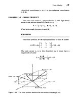
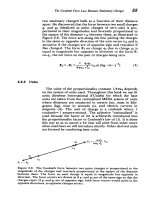
Figure
2-6
The
Coulomb
force
between
two
point
charges
is
proportional
to
the
magnitude
of
the
charges
and
inversely
proportional
to
the

square
of
the
distance
between
them.
The
force
on
each
charge
is
equal
in
magnitude
but
opposite
in
direction.
The
force
vectors
are
drawn
as
if
q,
and
q
2

,
are
of
the
same
sign
so
that
the
charges
repel.
If
q,
and
q
2
are
of
opposite
sign,
both
force
vectors
would
point
in
the
opposite
directions,
as

opposite
charges
attract.
56
The
Electric
Field
The
parameter
Eo
is
called
the
permittivity
of
free
space
and
has
a
value
e0
=
(4rT
X
10-7C
2
)
- 1
10

- 9
-
9=
8.8542
x 10
- 1 2
farad/m
[A
2
-s
4
-
kg
-
_
m
-
3]
(2)
3 6
7r
where
c
is
the
speed
of
light
in
vacuum

(c
-3
x
10"
m/sec).
This
relationship
between
the
speed
of
light
and
a
physical
constant
was
an
important
result
of
the
early
electromagnetic
theory
in
the
late
nineteenth
century,

and
showed
that
light
is
an
electromagnetic
wave;
see
the
discussion
in
Chapter
7.
To
obtain
a
feel of
how
large
the
force
in
(1)
is,
we
compare
it
with
the gravitational

force
that
is
also
an
inverse
square
law
with
distance.
The
smallest
unit
of
charge
known
is
that
of
an
electron
with
charge
e
and
mass
me
e
-
1.60

x
10
- 19
Coul,
m,
_9.11
x
10
- •
kg
Then,
the ratio
of electric
to
gravitational
force
magnitudes
for
two
electrons
is
independent
of
their
separation:
F,
eI/(4rEor
2
)
e2

142
F=
-
m2
2
-2
=
-4.16x
10
(3)
F,
Gm,/r
m,
4ireoG
where
G=6.67
10-11
[m
3
-s-2-kg-']
is
the gravitational
constant. This
ratio
is
so
huge
that
it
exemplifies

why elec-
trical
forces
often dominate
physical
phenomena.
The
minus
sign
is
used
in
(3)
because
the
gravitational
force
between
two
masses
is
always
attractive
while
for
two like
charges
the
electrical
force

is
repulsive.
2-2-3
The
Electric
Field
If
the
charge
q,
exists
alone,
it
feels
no
force. If
we
now
bring
charge
q2
within
the
vicinity
of
qj,
then
q2
feels
a

force
that
varies
in
magnitude
and
direction
as
it
is
moved
about
in
space
and
is
thus
a
way
of
mapping
out
the
vector
force
field
due
to
q,.
A

charge
other
than
q
2
would
feel
a
different
force
from
q2
proportional
to
its
own
magnitude and
sign.
It
becomes
convenient
to
work
with
the quantity
of
force
per
unit charge
that

is
called
the
electric
field,
because
this
quan-
tity
is
independent
of
the
particular
value
of
charge
used
in
mapping
the
force
field.
Considering
q
2
as
the
test
charge,

the
electric
field
due
to
q,
at
the
position
of
q2
is
defined
as
F
o
•7
E
2
=
lim
,
' i
2
volts/m
[kg-m-s
- A ]
q
2
-O

q2
4qeor,
2
The
Coulomb
Force
Law
Between
Stationary
Charges
In
the definition
of
(4)
the
charge
q,
must
remain
stationary.
This requires
that
the
test
charge
q
2
be
negligibly
small

so
that
its
force on
qi
does
not
cause
q,
to
move. In
the
presence
of
nearby
materials,
the
test
charge
q
2
could
also
induce
or
cause
redistribution
of
the
charges

in
the
material.
To
avoid
these
effects
in
our
definition
of
the
electric
field,
we
make
the
test
charge
infinitely
small
so its
effects
on
nearby
materials
and
charges
are
also

negligibly
small.
Then
(4) will
also
be
a
valid
definition
of
the
electric
field
when
we
consider
the
effects
of
materials.
To
correctly
map the
electric
field,
the
test
charge
must
not

alter
the
charge
distribution
from
what
it
is
in
the
absence of
the
test
charge.
2-2-4
Superposition
If
our
system
only
consists
of
two
charges,
Coulomb's
law
(1)
completely describes
their
interaction and

the
definition
of
an
electric
field
is
unnecessary.
The
electric
field
concept
is
only
useful
when
there
are
large
numbers
of
charge
present
as
each
charge
exerts
a
force on
all

the
others.
Since
the
forces
on
a
particular
charge
are
linear,
we
can
use
superposition,
whereby
if
a
charge
q,
alone
sets
up
an
electric
field
El,
and
another
charge

q
2
alone
gives
rise
to
an electric
field
E
2
,
then
the
resultant
electric
field
with
both
charges
present
is
the
vector
sum
E
1
+E
2
.
This

means
that
if
a
test
charge
q,
is
placed
at
point
P
in
Figure
2-7,
in
the
vicinity
of
N
charges
it
will
feel
a
force
F,
=
qpEp
(5)

E
2
.
.
. .
.
. .
. . .
.
.
.

. .
.

.:·:·%
q
.

:::::
: : :::::::::::::::::::::::::::::::::::::::::::"
-
::::::::::::::::::::: :::
:::
::::




*

. .

q E
2
.
+E
":

,
" :.
ql,41q2,
q3

.
qN:::::::::::
Ep
El +
E2
+ +
E
+E
Figure
2-7
The
electric
field
due
to
a

collection
of
point
charges
is
equal
to
the
vector
sum
of
electric
fields
from
each
charge
alone.
58
The
Electric
Field
where
Ep
is
the
vector
sum
of
the
electric

fields
due
to
all
the
N-point
charges,
q
ql.
92.
3.
N.
Ep=
-2-
1+-_-12P+
P
2SP
+
2'
+
2ENP
E
4ieo
rlp
r2 p
rP
NP
=
'
Eqi,1-

(6)
Note
that
Ep
has
no
contribution
due
to
q,
since
a
charge
cannot
exert
a
force
upon
itself.
EXAMPLE
2-1
TWO-POINT
CHARGES
Two-point
charges
are
a
distance
a
apart

along
the
z
axis
as
shown
in
Figure
2-8.
Find the
electric
field
at
any
point
in
the
z = 0
plane
when
the
charges
are:
(a)
both
equal
to
q
(b)
of

opposite
polarity
but
equal
magnitude
+
q.
This
configuration
is
called
an
electric
dipole.
SOLUTION
(a)
In
the
z = 0
plane,
each
point
charge
alone
gives
rise
to
field
components
in

the
i,
and
i,
directions. When
both
charges
are
equal,
the
superposition
of
field
components
due
to
both
charges
cancel
in
the
z
direction
but
add
radially:
q
2r
E(z
=

0)
=
2
/2
47Eo
0
[r
+(a/2)
2
]
3
/
2
As
a
check,
note
that
far
away
from the
point
charges
(r
>>
a)
the
field
approaches that
of

a
point
charge
of
value
2q:
2q
lim
E,(z
=
0)
=
r.a
4rEor
2
(b)
When
the
charges
have
opposite
polarity,
the
total
electric
field
due
to
both
charges

now cancel
in
the
radial
direction
but
add
in
the
z
direction:
-q
a
E,(z
=
O)=
-q
2
)2]31
4
1Tso
[r
+(a/2)
2
]
2
Far
away
from
the

point
charges
the
electric
field
dies
off as
the
inverse
cube
of distance:
limE,(z
=
0)=
-qa
ra
47rEor
I
Charge
Distributions
59
[ri,
+
-
i'
]
[r
2
+
(+

)2
1/2
+ E2=
q
2r
E,2
[ri,

Ai,
1)2j
[r2
+(1)
2
11/2
-qa
r
2
+(
)23/2
(2
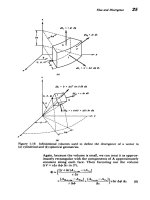
Figure
2-8
Two
equal
magnitude point
charges
are
a
distance
a

apart
along the
z
axis.
(a)
When
the charges
are
of the
same
polarity,
the
electric
field
due
to
each
is
radially
directed
away.
In
the
z
=
0
symmetry
plane,
the
net

field
component
is
radial.
(b)
When
the
charges are
of
opposite
polarity,
the
electric
field
due
to
the
negative
charge
is
directed
radially
inwards.
In
the
z
=
0
symmetry plane,
the net

field
is
now -z
directed.
The
faster rate
of
decay of
a
dipole
field
is
because
the
net
charge
is
zero
so
that
the
fields
due
to
each
charge
tend
to
cancel
each

other
out.
2-3
CHARGE
DISTRIBUTIONS
The
method
of
superposition
used
in
Section
2.2.4
will
be
used
throughout
the
text
in
relating
fields
to
their
sources.
We
first
find
the
field

due
to
a
single-point
source.
Because
the
field
equations
are
linear,
the net
field
due
to
many
point
2
60
The
Electric
Field
sources
is
just
the
superposition
of
the
fields

from
each
source
alone.
Thus,
knowing
the
electric
field
for
a
single-point
charge'at
an
arbitrary
position
immediately
gives
us
the
total
field
for
any
distribution
of
point
charges.
In
typical

situations,
one
coulomb
of
total
charge
may
be
present
requiring
6.25
x
108
s
elementary
charges
(e -
1.60x
10-'
9
coul).
When
dealing
with
such
a
large
number of
par-
ticles,

the
discrete
nature
of
the
charges
is
often
not
important
and
we
can
consider
them
as a
continuum.
We
can
then
describe
the charge
distribution
by
its
density.
The
same
model
is

used
in
the
classical
treatment
of
matter.
When
we
talk
about
mass
we
do
not
go to
the
molecular
scale
and
count
the
number
of
molecules,
but
describe
the
material
by

its
mass
density
that
is
the
product
of
the
local
average
number
of
molecules
in
a
unit
volume
and
the
mass
per
molecule.
2-3-1
Line,
Surface,
and
Volume
Charge
Distributions

We
similarly
speak of
charge
densities.
Charges
can
dis-
tribute
themselves
on
a
line
with
line
charge
density
A
(coul/m),
on
a
surface
with
surface
charge
density
a
(coul/m
2
)

or
throughout
a
volume
with
volume
charge
density
p
(coul/mS).
Consider
a
distribution
of
free charge
dq
of
differential
size
within
a
macroscopic
distribution
of
line,
surface,
or
volume
charge
as

shown
in
Figure
2-9.
Then,
the
total
charge
q
within
each
distribution
is
obtained
by
summing
up
all
the
differen-
tial
elements.
This
requires
an
integration
over
the
line,
sur-

face,
or
volume
occupied
by
the charge.
A
dl
J
A
dl
(line
charge)
dq=
adS
q=
s
r
dS
(surface
charge)
(1)
pdV
IJp
dV
(volume
charge)
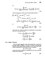
EXAMPLE
2-2
CHARGE

DISTRIBUTIONS
Find
the
total
charge
within
each of
the
following
dis-
tributions
illustrated
in
Figure
2-10.
(a) Line
charge
A
0
uniformly
distributed
in
a
circular
hoop
of
radius
a.
·_
Charge

Distributions
Point charge
(a)
t0j
dq
=
o
dS
q
=
odS
S
4-
4-
S
P
rQp
q
dq
=
Surface
charge
Volume
charge
(c)
(d)
Figure
2-9
Charge
distributions.

(a)
Point charge;
(b)
Line
charge;
(c)
Surface
charge;
(d)
Volume
charge.
SOLUTION
q=
Adl
=
Aoa
d
=
21raAo
(b)
Surface
charge
uo
uniformly
distributed
on
a
circular
disk
of

radius
a.
SOLUTION
a 2w
q=
odS=
1:-
J=0
0
or
dr
do
=
7ra
2
0
(c)
Volume
charge
po
uniformly
distributed
throughout
a
sphere
of
radius
R.
a
62

The
Electric
Field
y
ao
a+
+
-+
++
±
++_-
+
+f+
(a)
+
±
+
+
+
++
++
+
X
A
0
a
e-2r/a
1ra
3
Figure

2-10
Charge distributions
of Example
2-2.
(a)
Uniformly
distributed
line
charge
on
a
circular
hoop.
(b)
Uniformly
distributed
surface
charge
on
a
circular
disk.
(c)
Uniformly
distributed
volume
charge
throughout
a
sphere.

(d)
Nonuniform
line
charge
distribution.
(e)
Smooth
radially
dependent
volume
charge
distribution
throughout
all
space,
as
a
simple
model
of
the
electron
cloud
around
the
positively
charged
nucleus
of
the

hydrogen
atom.
SOLUTION
q =
=pdV
=
0
*V
=0-0=of
por
sin
0
dr
dO
do
=
3rrR
po
(d)
A
line
charge
of
infinite
extent
in
the
z
direction
with

charge
density
distribution
A
0
A-
+(z2]
SOLUTION
q
=
A
dl
A,
1
-
Aoa
tan
=
Aoi-a
q
j
[1+
(z/a)2]
a
I
-
Charge
Distributions
63
(e)

The
electron
cloud
around
the
positively
charged
nucleus
Q
in
the
hydrogen
atom
is
simply
modeled
as
the
spherically symmetric
distribution
p(r)=
-
e-2-
a
7ra
where
a
is
called
the

Bohr radius.
SOLUTION
The
total
charge
in
the
cloud
is
q=
f
p
dV
-
i=
-
sa
e-
'2r
sin
0
drdO
d
r=0
1=0
JO=O
=0ir
=
Lo
a

3e-2r/a
r2
dr
4Q
-2,/a
2
2
OD
- -~
e
[r
1)]
0
=-Q
2-3-2
The
Electric
Field
Due
to
a
Charge
Distribution
Each
differential
charge
element
dq
as
a

source
at
point
Q
contributes
to
the
electric
field
at.
a
point
P
as
dq
dE=
2
iQp
(2)
41rEorQp
where
rQp
is
the
distance
between
Q
and
P
with

iqp
the unit
vector
directed
from
Q
to
P.
To
find
the
total
electric
field,
it
is
necessary
to
sum
up
the
contributions
from
each
charge
element.
This
is
equivalent
to

integrating
(2)
over
the
entire
charge
distribution, remembering
that
both
the
distance
rQp
and
direction
iQp
vary
for
each
differential
element
throughout
the
distribution
E
2=
q
Q
(3)
111,q
-'7rEorQP

where
(3) is
a
line
integral
for
line
charges
(dq
=A
dl),
a
surface
integral
for
surface
charges
(dq
=
o-dS),
a
volume
64
The
Electric
Field
integral
for
a
volume

charge
distribution
(dq
=p
dV),
or
in
general,
a
combination
of
all
three.
If
the
total
charge
distribution
is
known,
the
electric
field
is
obtained
by
performing
the
integration
of

(3).
Some
general
rules
and
hints
in
using
(3)
are:
1.
It
is
necessary
to
distinguish
between
the
coordinates
of
the
field
points
and
the charge
source
points.
Always
integrate
over

the coordinates
of
the
charges.
2.
Equation
(3) is
a
vector
equation and
so
generally
has
three
components
requiring
three
integrations.
Sym-
metry
arguments
can
often
be
used
to
show
that
partic-
ular

field
components
are
zero.
3.
The
distance
rQp is
always
positive.
In
taking
square
roots,
always
make
sure
that
the
positive
square
root
is
taken.
4.
The
solution
to
a
particular

problem
can
often
be
obtained
by
integrating
the
contributions
from
simpler
differential
size
structures.
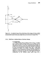
2-3-3
Field
Due
to an
Infinitely
Long
Line
Charge
An
infinitely
long
uniformly
distributed
line
charge
Ao

along the
z
axis
is
shown
in
Figure
2-11.
Consider the
two
symmetrically
located
charge
elements
dq
1
and
dq
2
a
distance
z
above
and
below
the
point
P,
a
radial

distance
r
away.
Each
charge
element
alone
contributes
radial
and
z
components
to
the
electric
field.
However,
just
as
we
found
in Example
2-la,
the
two
charge
elements
together
cause
equal

magnitude
but
oppositely
directed
z field
components
that thus
cancel
leav-
ing
only
additive
radial
components:
A
0
dz
Aor
dz
dEr=
4
(z
+
r)
cos
0
=
4ireo(z
2
+

/2
(4)
To
find
the
total
electric
field
we
integrate
over
the
length
of
the
line
charge:
Aor
I_
dz
4rreo
J-
(z+r
)/2
A
0
r
z
+
Go

41re
0
r
2
(z
2
+r
+
2
)
/
=-
2
2reor
Ar