Electromagnetic Field Theory: A Problem Solving Approach Part 10 ppsx

Charge
Distributions
dqi
=
Xodz
+
z
2
)1/2
+
dE
2
dE,
dq2
=
Xo
dz
Figure
2-11
An
infinitely
long
uniform
distribution
of
line
charge
only
has
a
radially

directed
electric
field
because
the
z
components
of
the
electric
field
are
canceled
out
by
symmetrically
located
incremental
charge
elements
as
also
shown
in
Figure
2-8a.
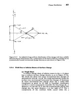
2-3-4
Field
Due
to

Infinite
Sheets
of
Surface
Charge
(a)
Single
Sheet
A
surface
charge
sheet
of
infinite
extent
in
the
y
=
0
plane
has
a
uniform
surface
charge
density
oro
as
in

Figure
2-12a.
We
break
the
sheet
into
many
incremental
line
charges
of
thickness
dx
with
dA
=
oro
dx.
We
could
equivalently
break the
surface
into
incremental
horizontal
line
charges
of

thickness
dz.
Each
incremental
line
charge
alone
has
a
radial
field
component
as
given
by
(5)
that
in
Cartesian
coordinates
results
in
x
and
y
components. Consider
the
line
charge
dA

1
, a
distance
x
to
the
left
of
P,
and
the
symmetrically
placed
line
charge
dA
2
the
same
distance
x
to
the
right
of
P.
The
x
components
of

the
resultant
fields cancel
while
the
y
The
Electric
Field
00
2
(0
o
2•'•
oo/eo
1 11
2
III
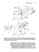
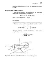
Figure
2-12
(a)
The
electric
field
from
a
uniformly
surface
charged
sheet

of
infinite
extent
is
found
by
summing the
contributions
from
each
incremental
line
charge
element.
Symmetrically
placed
line
charge
elements
have
x
field
components
that
cancel,
but
y
field
components
that

add.
(b)
Two parallel
but
oppositely
charged
sheets
of
surface
charge
have
fields
that
add
in
the
region
between
the
sheets
but
cancel
outside.
(c)
The
electric
field
from
a
volume

charge
distribution
is
obtained
by
sum-
ming
the
contributions from
each
incremental
surface
charge
element.
x
00
2eo
-t-
oo
woo
Charge
Distributions
do
= pody'
'S
ijdy'
p.:
."P0
"
,-'

II'.
":i : :,:
a
a
po
0
a
'o
components
add:
Eo
dx
aoy
dx
dE,
=
o(
+
cos
0
=
(+y)
21reo(x2+y
)
2
27eo(x2
+y2)
The
total
field

is
then
obtained
by
integration
over
all
line
charge
elements:
+aO
E
roY
or
dx
Ey
J
2
2
S21rEo
x
+y
=

y
tan-
2
rEo
yy
y1

-rn
So/2eo,
y>O
0
-o'o/2Eo,
y
<0
where
we
realized
that the
inverse
tangent
term
takes
the
sign
of
the
ratio
x/y
so
that
the
field
reverses
direction
on
each
side

of
the
sheet.
The
field
strength
does
not
decrease
with
dis-
tance
from
the
infinite
sheet.
(b)
Parallel
Sheets
of
Opposite
Sign
A
capacitor
is
formed
by
two
oppositely
charged

sheets
of
surface
charge
a
distance
2a apart
as
shown
in
Figure
2-12b.
III
Po0
dy'
dE
=
P
I
dE=

O
-
Fig.
212()o
Fig.
2-12(c)
:
·
··

jr
: ·
: ·
: ·:
: ·
C r-
/I
V
=
_V
tJ
68
The
Electric
Field
The
fields
due
to
each
charged
sheet
alone
are
obtained
from
(7)
as
y,,
y>-

a

,
y>a
2Eo
2EO
E
i=
E2
(8)
ro.
To
.
-
,,
y <-a
,i,
y<a
2EO
2EO
Thus,
outside
the
sheets
in
regions
I
and
III
the

fields
cancel
while
they
add
in
the
enclosed
region
II.
The
nonzero
field
is
confined
to
the region
between
the
charged
sheets
and
is
independent
of
the
spacing:
E
=
E,+E

2
=
(
IyI>a
(9)
0
jy|
>a
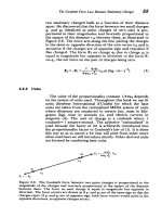
(c)
Uniformly Charged
Volume
A
uniformly charged
volume
with
charge
density
Po
of
infinite
extent
in
the
x
and
z
directions
and
of
width 2a

is
centered
about
the
y
axis,
as
shown
in
Figure
2-12c. We
break
the
volume
distribution
into
incremental
sheets
of
surface
charge
of
width
dy'
with
differential surface
charge
density
do-
=

Po
dy'.
It
is
necessary
to
distinguish
the
position
y'
of
the
differential
sheet
of
surface
charge from
the
field
point
y.
The
total
electric
field
is
the
sum
of
all

the
fields
due
to
each
differentially
charged
sheet.
The
problem
breaks
up
into
three
regions.
In
region
I,
where
y
5
-a,
each
surface
charge
element
causes
a
field in
the

negative
y
direction:
E,=
2dy
=
pa
y
-
a
(10)
a
2eo
60
Similarly,
in
region
III,
where
y >
a,
each
charged sheet
gives
rise to
a
field in
the
positive
y

direction:
E
Po
yya
(11)
E
fa
PO
,
=
poaa
y
>
a
(11)
-a
2Eo
Eo
For
any
position
y
in
region
II,
where
-a
y
5
a,

the
charge
to
the
right
of
y
gives
rise
to
a
negatively
directed
field
while
the
charge
to
the
left of
y
causes
a
positively
directed
field:
I
Pody'
a
P

oy
E,=
2E+
(-)
dy'o -, -ao
y5a
(12)
2
2eo
8o
The
field
is
thus constant
outside
of
the
volume
of
charge
and
in
opposite
directions
on
either
side
being
the
same

as
for
a
Charge
Distributions
69
surface
charged
sheet
with
the
same
total
charge
per
unit
area,
0o
=
po2a.
At
the
boundaries
y
=
±a,
the
field is
continuous,
changing

linearly
with
position
between
the
boundaries:
poa

L,
y

a
E,
=
o,
-a
-y
-
a
(13)
so
poa
,
y>-a
6
,O0
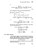
2-3-5
Superposition
of
Hoops

of
Line
Charge
(a)
Single
Hoop
Using
superposition,
we
can similarly
build
up
solutions
starting
from
a
circular
hoop
of
radius
a
with
uniform
line
charge
density
A
0
centered
about

the origin
in
the
z =
0
plane
as
shown
in
Figure
2-13a.
Along
the
z
axis,
the
distance
to
the
hoop
perimeter
(a2+z2)
1
1
2
is
the
same
for
all

incremental
point
charge
elements
dq
=
Aoa
d.
Each
charge
element
alone
contributes
z-
and
r-directed
electric
field
components.
However,
along
the
z
axis
symmetrically
placed
elements
180*
apart
have

z
components
that
add
but
radial
components
that
cancel.
The
z-directed
electric
field
along
the
z
axis
is
then
E
f2w
Aoa
d4
cos
0
Aoaz
E2=
2
2
2 -

(14)
47rEo(z
+a
)
2eo(a
+Z2
The
electric
field
is
in
the
-z
direction along
the
z
axis
below
the
hoop.
The
total
charge
on the
hoop
is
q
=
27taXo
so

that
(14)
can
also
be
written
as
qz
E.=
4reo(a
+z )
3
/
2
(15)
When
we
get
far
away
from
the
hoop
(IzI >
a),
the
field
approaches
that
of

a
point charge:
q
Jz>0
lim
Ez
= ± 2
z0
(16)
I%1
*a
t4rEoz
z<0
(b)
Disk
of
Surface
Charge
The
solution
for
a
circular
disk
of
uniformly
distributed
surface
charge
Oo

is
obtained
by
breaking
the
disk
into
incremental
hoops
of
radius
r
with
line
charge
dA
=
oo
dr
as
in
70
The
Electric
Field
a
rouup
01 llr
ulnargyr
Ui

o
surlace
Lhargy
of
(c)
(d)
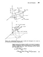
Figure
2-13
(a)
The
electric
field
along
the
symmetry
z
axis
of
a
uniformly
dis-
tributed
hoop
of
line
charge
is
z
directed.
(b)

The
axial
field
from
a
circular
disk
of
surface
charge
is
obtained
by
radially
summing
the
contributions
of
incremental
hoops
of
line
charge.
(c)
The
axial
field
from
a
hollow

cylinder
of
surface
charge
is
obtained
by
axially
summing
the
contributions
of
incremental
hoops
of
line
charge.
(d)
The
axial
field
from
a
cylinder
of volume
charge
is
found
by
summing

the
contributions
of
axial
incremental
disks
or
of
radial
hollow
cylinders of
surface
charge.
Figure
2-13b.
Then
the
incremental
z-directed
electric
field
along
the
z
axis
due
to
a
hoop
of

radius
r
is
found
from
(14)
as
o=
orz
dr
dE=
2e(r
2
+z
2
)
2
(17)
2)P12
Y
•v
Charge
Distributions
71
where
we
replace
a
with
r,

the
radius
of
the
incremental
hoop.
The
total
electric
field
is
then
a
rdr
Io_
2
2t
32
=
2eo
J
(r
+z
)
o1oz
2eo(r
2
+z
2
)1I

2
0
•(o
z z
2EO
(a2
+2
1/2
IZI
2e,
'(a
+z)u
2
I|z|
ro
roz
z > 0
2Eo
20(a
2
2
1/2
z<
where care
was
taken
at
the
lower
limit

(r
=
0),
as
the
magni-
tude
of
the
square
root
must
always
be
used.
As
the
radius
of
the
disk
gets
very
large,
this
result
approaches
that
of
the

uniform
field
due
to
an
infinite
sheet
of
surface charge:
lim
E.
=
>0
(19)

002oo
z
<0
(c)
Hollow
Cylinder
of
Surface Charge
A
hollow
cylinder
of
length
2L
and

radius
a
has
its axis
along
the
z
direction
and
is
centered about
the
z =
0
plane
as
in
Figure
2-13c.
Its
outer
surface
at
r=a
has
a
uniform
distribution
of
surface

charge
0o.
It
is
necessary
to
distinguish
between
the
coordinate
of
the
field
point
z
and
the
source
point
at
z'(-L
sz':-L).
The
hollow
cylinder
is
broken
up
into
incremental

hoops
of
line
charge
dA
=
o
0
dz'.
Then,
the
axial
distance
from
the
field
point
at
z
to
any
incremental
hoop
of
line
charge
is
(z
-z').
The

contribution
to
the
axial
electric
field
at
z
due
to
the incremental
hoop
at
z'
is
found
from
(14)
as
E=
oa
(z -
z')
dz'
dE=
2e[a
2+
(z
-z')
2

]
31
(20)
which
when
integrated
over
the length
of
the
cylinder
yields
o
a
+L
(z
-z')dz'
Ez
2e
J-L
[a
2
+
(z
-
z')
2
1
2
=ooa

1
+L
2eo
[a
2
+
(z
-
z'
)
2
]
/2'
o
\[a
2
+(z
L)2]1/2
[a2+(Z
+L)211/2)
(21)
p• -,,,•r
72
The
Electric
Field
(d)
Cylinder
of
Volume

Charge
If
this same
cylinder
is
uniformly
charged
throughout
the
volume
with
charge
density
po,
we
break
the
volume
into
differential-size
hollow
cylinders
of
thickness
dr
with
incre-
mental
surface
charge

doa
=
po
dr
as
in
Figure
2-13d.
Then,
the
z-directed
electric
field
along
the
z
axis
is
obtained
by
integra-
tion
of
(21)
replacing
a
by
r:
P
1 1

E,
-
r 9I
r2
21/2
2
2
112J
dr
=
0
a
r(
2(
1L)],,)
dr
2e
0
Jo
r[r
+(z
-L)]l/[r
+(z+L)I
=
P•
{[r2
+ (Z-
L)2]1/2-[r2
+ (Z +
L2)]1/2}1

2eo
+Iz+LL}
(22)
where
at
the
lower
r=
0
limit
we
always
take
the
positive
square
root.
This
problem
could
have
equally
well
been
solved
by
breaking
the
volume
charge

distribution
into
many
differen-
tial-sized
surface
charged
disks
at position
z'(-L
-z'-L),
thickness
dz',
and
effective
surface
charge
density
do
=
Po
dz'.
The
field
is
then
obtained
by
integrating
(18).

2-4 GAUSS'S
LAW
We
could
continue
to
build
up
solutions
for
given
charge
distributions
using the
coulomb
superposition
integral
of
Section
2.3.2.
However,
for
geometries
with
spatial
sym-
metry,
there
is
often

a
simpler
way
using
some
vector
prop-
erties of
the
inverse
square
law
dependence
of
the
electric
field.
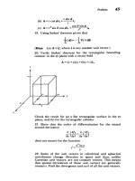
2-4-1
Properties of
the
Vector
Distance
Between
Two
Points,
rop
(a)
rp
In
Cartesian

coordinates
the
vector
distance
rQp
between
a
source
point
at
Q
and
a
field
point
at
P
directed
from
Q
to
P
as
illustrated
in
Figure
2-14
is
rQp
=

(x
-
Q)i
2
+
(y
-
yQ)i,
+
(z
-
zQ)i'
(1)
with
magnitude
rQp
=
[(x
-xQ)
+
(yY
-yQ)2
+
(z
-
zQ)
]]
• 2
(2)
The

unit
vector
in
the
direction
of
rQP
is
fr
rQP
QP
iO_.
Gauss's
Law
73
2
x
Figure
2-14
The
vector
distance
rQp
between
two
points
Q
and
P.
(b)

Gradient
of
the
Reciprocal
Distance,
V(l/rQp)
Taking
the
gradient
of
the
reciprocal
of
(2)
yields
V
I
=
j-2
I
+
,
a
I
a
rQ
ax
ro
,
y

r,)
az
rQ
1
=
r- [(x
-XQ)i:
+ (Y
-YQ)i,
+
(z
-
zQ)iz]
rQP
=
-iQp/rQP
(4)
which
is
the
negative
of
the
spatially
dependent
term
that
we
integrate
to

find
the
electric
field
in
Section
2.3.2.
(c)
Laplacian
of
the
Reciprocal
Distance
Another
useful identity
is
obtained
by
taking
the
diver-
gence
of
the
gradient
of
the
reciprocal
distance.
This opera-

tion
is
called
the
Laplacian
of
the
reciprocal distance.
Taking
the divergence
of
(4)
yields
S QP
3
3
(

+ [(x-xQ)
2
+(y-y
Q)
2
+(z
zQ)]
(5)
rQp
rQ
y
y

74
The Electric
Field
Using
(2)
we
see
that
(5)
reduces
to
2
_
= O,
rq,
O0
rQp
(6)
rQp)
=undefined
rQp=
0
Thus,
the
Laplacian
of
the
inverse
distance
is

zero
for
all
nonzero
distances
but
is
undefined
when
the
field
point
is
coincident
with
the source
point.
2-4-2
Gauss's
Law
In
Integral
Form
(a)
Point
Charge
Inside
or
Outside
a

Closed Volume
Now
consider the
two
cases
illustrated
in
Figure
2-15
where
an
arbitrarily
shaped
closed
volupne
V
either
surrounds
a
point
charge
q
or
is
near
a
point
charge
q
outside the

surface
S.
For
either
case
the
electric
field
emanates
radially
from
the
point
charge
with
the
spatial
inverse
square
law.
We
wish
to
calculate
the
flux
of
electric
field
through

the
surface
S
sur-
rounding
the
volume
V:
=
sE
-
dS
=•s
4
or
2
PiQpdS
%
eorp7)
-qv
=S
41r
o
(rQP)
d S
(7)
#
oE
dS=
f

oE
dS=q
S
S'
dS
(a)
(b)
Figure
2-15
(a)
The
net
flux
of
electric
field
through
a
closed
surface
S
due
to
an
outside
point
charge
is
zero
because

as
much
flux
enters
the
near
side
of
the
surface
as
leaves
on
the
far
side.
(b)
All
the
flux
of
electric
field
emanating
from
an
enclosed
point
charge
passes

through
the
surface.