Electromagnetic Field Theory: A Problem Solving Approach Part 23 pdf

Lossy
Media
195
p
(x
=
0)
=
Po
, 1
PU
-T-
P1
W
ý poe
x1AM
=E
apIm
I
Figure
3-25
A
moving
conducting
material
with
velocity
Ui,
tends
to
take

charge
injected
at
x
=0
with
it.
The
steady-state
charge
density
decreases
exponentially
from
the
source.
velocity
becomes
dpf,
a
d+p
+"a
P
=
0
(56)
dx
EU
which
has

exponentially
decaying
solutions
pf
=
Po e
- a
,
1=
(57)
where
1.
represents
a
characteristic
spatial
decay
length.
If
the
system
has
cross-sectional
area
A,
the
total
charge
q
in

the
system
is
q
=
pfA
dx
=
polA
(58)
3-6-6
The
Earth
and
its
Atmosphere
as
a
Leaky
Spherical
Capacitor*
In
fair
weather,
at
the
earth's
surface
exists
a

dc
electric
field
with
approximate
strength
of
100
V/m
directed
radially
toward
the
earth's
center.
The
magnitude
of
the
electric
field
decreases
with
height
above
the
earth's
surface
because
of

the
nonuniform
electrical
conductivity
oa(r)
of
the
atmosphere
approximated
as
cr(r)
=
ro
+
a(r
- R
)2
siemen/m
(59)
where
measurements
have shown
that
ro-
3
10-14
a
.5
x
10

-
2
0
(60)
*
M.
A.
Uman,
"The
Earth
and
Its
Atmosphere
as
a
Leaky
SphericalCapacitor,"Am.
J.
Phys.
V.
42,
Nov.
1974,
pp.
1033-1035.
196
Polarization
and
Conduction
and

R
-6
x
106
meter
is
the
earth's
radius.
The
conductivity
increases
with
height
because
of
cosmic
radiation
in
the
lower
atmosphere.
Because
of
solar
radiation
the
atmosphere
acts
as a

perfect
conductor
above
50
km.
In
the
dc
steady
state,
charge
conservation
of
Section
3-2-1
with
spherical symmetry
requires
18 C
VJ=
(rJ,)
=
>
J, =
(r)E,
=
(61)
r2
8r
r

where
the constant
of
integration
C
is
found
by
specifying
the
surface
electric
field
E,(R)*
-
100
V/m
O(R)E,(R)R
2
J,(r)
=
2
(62)
At
the
earth's
surface
the
current
density

is
then
J,(R)
=
o(R)E,(R)
=
roE,(R)

3
x
10-12
amp/m2
(63)
The
total
current
directed
radially
inwards over
the
whole
earth
is
then
I
=
IJ,(R)47rR
2
1 - 1350
amp

(64)
The
electric
field
distribution
throughout
the
atmosphere
is
found
from
(62)
as
J
,
(r )
=(R)E,(R)R2
E,(r)
2(r)
(65)
o(r)
r
o(r)
The
surface
charge
density
on
the
earth's

surface
is
(r
=
R)
=
EoE,(R)
-
-8.85
x
10
- 1
'
Coul/m
2
(66)
This
negative
surface
charge
distribution
(remember:
E,(r)
<
0)
is
balanced
by
positive
volume

charge
distribution
throughout
the
atmosphere
Eo
2
soo(R)E,(R)R
2
d
1
p,(r)=
eoV
-
E=
r (rE,)=
2
L\(
r~r
22
r
dr
o(r)
S-soo(R)E,(R)R
2
(67)
r2((r))
2a(r-R)
The
potential

difference
between
the
upper
atmosphere
and
the
earth's
surface
is
V=
J-
E,(r)dr
o(R)E(R)2r
2[o[o+a(r-R)
2
]
Field-dependent
Space
Charge
Distributions
197
1
(R2
t)
r(R
2
)
+
C10(R+'2

)2
( 1
a
l
a
r(R)E,(R)
a(R'
+ 0)'
Using
the
parameters
of
(60), we
see
that
rola
<<
R
2
so
that
(68)
approximately reduces
to
aR
2
aR
2
IoE,(R)
n

(69)
-
384,000
volts
If
the
earth's
charge
were
not
replenished,
the
current
flow
would
neutralize
the
charge
at
the
earth's
surface
with
a
time
constant of
order
£0
7 =
-=

300
seconds
(70)
0o
It
is
thought
that
localized
stormy regions
simultaneously
active
all
over
the
world
serve
as
"batteries"
to
keep
the
earth
charged
via
negatively
chairged
lightning
to
ground

and
corona
at
ground
level,
producing
charge
that
moves
from
ground
to
cloud.
This
thunderstorm
current
must
be
upwards
and
balances
the
downwards
fair
weather
current
of
(64).
3.7
FIELD-DEPENDENT

SPACE
CHARGE
DISTRIBUTIONS
A
stationary
Ohmic
conductor
with
constant
conductivity
was
shown
in
Section
3-6-1
to
not
support
a
steady-state
volume
charge
distribution.
This
occurs
because
in
our
clas-
sical

Ohmic
model
in
Section
3-2-2c
one
species
of
charge
(e.g.,
electrons
in
metals)
move
relative
to
a
stationary
back-
ground
species
of
charge
with
opposite
polarity
so
that
charge
neutrality

is
maintained.
However,
if
only
one
species
of
(68)
198
Polarization
and
Conduction
charge
is
injected
into
a
medium,
a
net
steady-state
volume
charge
distribution
can
result.
Because
of
the

electric
force,
this
distribution
of
volume
charge
py
contributes
to
and
also
in
turn
depends
on
the
electric
field.
It
now
becomes
necessary
to
simultaneously
satisfy
the
coupled
electrical
and

mechanical
equations.
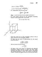
3-7-1
Space
Charge
Limited
Vacuum
Tube Diode
In
vacuum
tube
diodes, electrons
with
charge
-e
and
mass
m
are
boiled
off
the
heated
cathode,
which
we
take
as
our
zero

potential
reference. This
process
is
called
thermionic
emis-
sion.
A
positive
potential
Vo
applied
to
the
anode
at
x
=
l
accelerates
the
electrons,
as
in
Figure
3-26.
Newton's
law
for

a
particular
electron
is
dv
dV
m
=
-
eE
=
e
(1)
dt
dx
In
the
dc
steady state
the
velocity
of
the
electron
depends
only
on
its
position
x

so
that
dv
dv
dx
dv
d
2
d
m-=
=
mymv (
)=
-(e
V)
(2)
dt
dx
dt
dx
dx
dx
V
0
+II
1ll
-e
+
2eV
1/

2
+
V=
[
- E
m
J
-Joix
+
=
JoA
Area
A
Cathode
Anode
I I - x
0
I
(a)
(b)
Figure
3-26
Space
charge
limited vacuum
tube diode.
(a)
Thermionic
injection
of

electrons
from
the
heated
cathode
into
vacuum
with
zero
initial
velocity.
The
positive
anode
potential
attracts the
electrons
whose
acceleration
is
proportional
to
the
local
electric
field.
(b)
Steady-state
potential,
electric

field,
and
volume
charge
distributions.
|Ill
0
1
Field-dependent
Space
Charge
Distributions
199
With
this
last
equality,
we
have
derived
the energy
conser-
vation
theorem
d
[mv
2
-eV]
=
O

mv
2
-
eV=
const
(3)
dx
where
we
say
that
the
kinetic
energy
2mv
2
plus
the
potential
energy
-eV
is
the
constant
total
energy.
We
limit
ourselves
here

to
the
simplest
case
where
the
injected
charge
at
the
cathode
starts
out
with
zero
velocity.
Since
the
potential
is
also
chosen
to
be
zero at
the
cathode, the
constant
in
(3) is

zero.
The
velocity
is
then
related
to
the
electric
potential
as
=
(2e
V)
I/
1/
(4)
In
the
time-independent
steady
state
the
current
density
is
constant,
dJx
JJ=O
-

O=J
=
-Joi.
(5)
dx
and
is
related
to
the
charge
density
and
velocity
as
In
1/2
o
=
-PfvjpJf
=
-JO(2e)
1 9
V
-
1
2
(6)
Note
that

the
current
flows
from
anode
to
cathode,
and
thus
is
in
the
negative
x
direction.
This
minus
sign
is
incorporated
in
(5)
and
(6)
so
that
Jo
is
positive.
Poisson's

equation then requires
that
V2V=
-P
dV
Jo
'm
1/2v-
\•eW
(7)
Power
law
solutions
to
this
nonlinear
differential
equation
are
guessed
of
the
form
V
=
Bx
(8)
which
when
substituted

into
(7)
yields
Bp(p
-
1)x
-2
=
o
(;
12
B-1/2X-02
(9)/
For
this
assumed
solution
to
hold
for
all
x
we
require
that
p
4
-2=
-p
=

(10)
2
3
which
then
gives
us
the amplitude
B
as
B
4=
[
/22/s
(11)
I
200
Polarization
and
Conduction
so
that
the
potential
is
V(x)-=
9'-
1
2
2Ex

4
(12)
The
potential
is
zero at
the
cathode,
as
required,
while
the
anode potential
Vo
requires
the
current
density
to
be
V(x
=
)
=
Vo
=
I
1/22/
4/3
4e

\2e
/2
/2
o
=
V;9
(13)
which
is
called
the
Langmuir-Child
law.
The
potential,
electric
field,
and
charge distributions
are
then
concisely
written
as
V(x)
=
Vo(!
)
dV(x)
4

Vo
(I\s
E(x)
=
- - )
(14)
dE(x)
4
Vo
(x)-
2
/s
and
are
plotted
in
Figure
3-26b.
We
see
that
the
charge
density
at
the
cathode
is
infinite
but

that
the
total
charge
between
the
electrodes
is
finite,
q-=
p(x)Adx=

ve-A
(15)
being
equal
in
magnitude
but
opposite
in sign
to
the
total
surface
charge
on
the
anode:
4Vo

qA=
of(x=1)A=
-eE(x=1)A=
+ -4-A
(16)
3
1
There
is
no surface
charge
on
the
cathode
because
the
electric
field
is
zero
there.
This
displacement
x
of
each
electron
can
be
found

by
substituting
the
potential
distribution
of
(14)
into
(4),
S(2eVo
2
(
)2/
is
dx
_
2eVo
,
1/2
v
- ~-5
=( 2
dt
(17)
which
integrates
to
x=
7iýi)
'

(18)
Field-dependent
Space
Charge
Distributions
201
The
charge
transit
time
7
between
electrodes
is
found
by
solving
(18)
with
x
=
1:
=
3(1
(19)
For
an
electron
(m
=

9.1
x
10
- s
'
kg,
e
=
1.6
10-'
9
coul)
with
100
volts
applied
across
1
=
1
cm
(10
-
2
m)
this
time
is
7~
5

x 10
- 9
sec.
The
peak electron
velocity
when
it
reaches
the
anode
is
v(x
=
1)-6x
106
m/sec,
which
is
approximately
50
times
less
than
the
vacuum
speed
of
light.
Because

of
these
fast
response
times
vacuum
tube
diodes
are
used
in
alternating
voltage
applications
for
rectification
as
current
only
flows
when
the
anode
is
positive
and
as
nonlinear
circuit
elements

because
of
the
three-halves
power
law
of
(13)
relating
current
and
voltage.
3-7-2
Space
Charge
Limited
Conduction
in
Dielectrics
Conduction
properties
of
dielectrics
are often
examined
by
injecting
charge.
In
Figure

3-27,
an
electron
beam
with
cur-
rent
density
J
=
-Joi,
is
suddenly
turned
on
at
t
=
0.*
In
media,
the
acceleration
of
the
charge
is
no
longer
proportional

to
the
electric
field.
Rather,
collisions
with
the
medium
introduce
a
frictional
drag
so
that
the
velocity
is
proportional
to
the
elec-
tric
field
through
the
electron
mobility
/A:
v

=
-AE
(20)
As
the
electrons
penetrate
the
dielectric,
the
space
charge
front
is
a
distance
s
from
the
interface
where
(20)
gives
us
ds/dt
=
-tE(s)
(21)
Although
the

charge
density
is
nonuniformly
distributed
behind
the
wavefront,
the
total
charge
Q
within
the
dielectric
behind
the
wave
front
at
time
t
is
related
to
the
current
density
as
JoA

=
pE.A
= -
Q/t
Q
=
-JoAt
(22)
Gauss's
law
applied
to
the
rectangular
surface
enclosing
all
the charge
within
the
dielectric
then
relates
the
fields
at
the
interface
and
the

charge
front
to
this
charge
as
E-
dS
=
(E(s)-oE(0)]A
=
Q
=
-JoAt
(23)
*
See
P.
K.
Watson,
J.
M.
Schneider,
and
H.
R.
Till,
Electrohydrodynamic
Stability
of

Space
Charge
Limited
Currents
In
Dielectric
Liquids.
IL.
Experimental
Study,
Phys.
Fluids
13
(1970),
p.
1955.
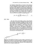
202
Polarization
and
Conduction
Electron
beam
A=
- 1-i
Space
charge
limited
Surface
of
integration

for
Gauss's
condition:
E(O)=0w:
Es-
A==-At
.
eo
law:
fE__
[(s)-eoE(OI]A=Q=-JoAe
- I
0
/
sltl
~+e-=
E
Moving
space
charge
front
Se,
p
=
0
E
=ds
Electrode
area
-Es)

7Electrode
area
A
Sjo
1/2
t
E•
j
=
Figure
3-27
(a)
An
electron
beam
carrying
a
current
-Joi,
is
turned
on
at
t
=
0.
The
electrons
travel
through

the
dielectric
with
mobility
gp.
(b)
The
space
charge
front,
at
a
distance
s
in
front
of
the
space
charge
limited
interface
at
x
=
0,
travels
towards
the
opposite

electrode.
(c)
After
the
transit
time
t,
=
[2el/IJo]
1
'
2
the
steady-state
potential,
electric
field,
and
space
charge
distributions.
The
maximum
current
flows
when
E(O)
=
0,
which

is
called
space
charge
limited
conduction.
Then
using
(23)
in
(21)
gives
us
the
time
dependence
of
the
space
charge
front:
ds
iJot
iLJot
2
=
O
s(t
)
=

dt
e 2e
Behind
the
front
Gauss's
law
requires
dE~,
P
Jo
dE.
Jo
-
=E
E
dE.
dx
e
eAE.
x
dx
EL-
(24)
(25)
~I
Field-dependent
Space
Charge
Distributions

203
while
ahead
of
the
moving
space
charge
the
charge
density
is
zero
so
that
the
current
is
carried
entirely
by
displacement
current
and
the
electric
field
is
constant
in

space.
The
spatial
distribution
of
electric
field
is
then
obtained
by
integrating
(25)
to
E•=
-I2JOx
, 0:xs(t)
(26)
-%2_Jos/e,
s(t)Sxli
while
the
charge
distribution
is
S=dE
-eJo/(2x),
O
-x s(t)
(27)

Pf=e
(27)
dx
0,
s(t):x5l
as
indicated
in
Figure
3-27b.
The
time
dependence
of
the
voltage
across
the
dielectric
is
then
v(t)
=
Edx
=
ojx
d+
-x
d
Jolt

Aj2t3
e
6
,
s(t)_l
(28)
6
6E2
These
transient
solutions
are
valid
until
the
space
charge
front
s,
given
by
(24),
reaches
the
opposite
electrode
with
s
=
I

at time
€
=
12-
e11to
(29)
Thereafter,
the
system
is
in
the
dc
steady
state
with
the
terminal
voltage
Vo
related
to
the
current
density
as
9
e;L
V2
Jo=

8-
(30)
8
1S
which
is
the
analogous
Langmuir-Child's
law
for
collision
dominated
media.
The
steady-state
electric
field
and
space
charge
density
are
then
concisely
written
as
3
Vo
2

dE
3E
V
0
1
(31)
2 1
dx-
4
1.
and
are plotted
in
Figure
3-27c.
In
liquids
a
typical
ion
mobility
is
of
the
order
of
10
-7
m
2

/(volt-sec)
with
a
permittivity
of
e
=
2e0
1.77Ox
10-
farad/m.
For
a
spacing
of
I=
O-2
m
with
a
potential
difference
of
Vo
=
10
V
the
current
density

of
(30)
is
Jo
2
10-4
amp/m
2
with
the transit
time
given
by
(29)
r
r0.133
sec.
Charge
transport
times
in collison
dominated
media
are
much
larger
than
in
vacuum.
204

Polarization
and
Conduction
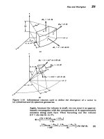
3-8
ENERGY
STORED
IN
A
DIELECTRIC
MEDIUM
The
work
needed
to
assemble
a
charge distribution
is
stored
as
potential
energy
in
the
electric
field
because
if
the
charges

are
allowed
to
move
this
work
can
be
regained
as
kinetic
energy
or
mechanical
work.
3-8-1
Work Necessary
to
Assemble
a
Distribution
of Point
Charges
(a) Assembling
the
Charges
Let
us
compute
the

work necessary
to
bring
three
already
existing
free
charges
qj,
q2,
and
qs
from
infinity
to
any
posi-
tion,
as
in
Figure
3-28.
It
takes
no
work
to
bring
in
the

first
charge
as
there
is
no
electric
field
present.
The
work
neces-
sary
to
bring
in
the
second
charge
must
overcome
the
field
due
to
the
first
charge,
while
the

work
needed
to
bring
in
the
third
charge
must
overcome
the
fields
due
to
both
other
charges.
Since
the
electric
potential
developed
in Section
2-5-3
is
defined
as
the
work
per

unit
charge
necessary
to
bring
a
point
charge
in
from
infinity,
the
total work
necessary
to
bring
in
the
three
charges
is
q,
\+
Iq__+
q2
W=q,()+q2r +qsl +
(1)
4
irer
2

l
'
4wer
15
4rrer
2
sl
where
the
final
distances
between
the
charges
are
defined
in
Figure
3-28
and
we
use
the
permittivity
e
of
the
medium.
We
can

rewrite
(1)
in
the more
convenient
form
W=
_[
q2
+
qs
+q
q,
+
3
2
4
4erel2
4erTsJ
, 4ITerl
2
4r823J
q
4q
+
2
(2)
14rer3s
47rer23s
I

/
/
/
/
/
/
I
/
/
/
p.
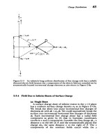
Figure
3-28
Three
already
existing
point
charges
are
brought
in
from
an
infinite
distance
to
their
final
positions.