Electromagnetic Field Theory: A Problem Solving Approach Part 29 pdf

Problems
255
(a)
What
is
the
time
dependence
of
the
dome
voltage?
(b)
Assuming
that
the
electric
potential
varies
linearly
between
the
charging
point and
the dome,
how
much
power
as
a
function

of
time
is
required
for
the
motor
to
rotate
the
belt?
-+++
R,
58.
A
Van de Graaff
generator
has
a
lossy
belt
with
Ohmic
conductivity
cr
traveling
at
constant
speed
U.

The
charging
point
at
z
=
0
maintains
a
constant
volume
charge
density
Po
on the
belt
at
z
=
0.
The
dome
is
loaded
by
a
resistor
RL
to
ground.

(a)
Assuming
only
one-dimensional
variations
with
z,
what
are the
steady-state
volume
charge,
electric
field,
and
current
density
distributions
on
the
belt?
(b)
What
is
the
steady-state
dome
voltage?
59.
A

pair
of
coupled
electrostatic
induction
machines
have
their
inducer
electrodes
connected
through
a
load
resistor
RL.
In
addition,
each
electrode
has
a
leakage
resistance
R
to
ground.
(a)
For
what

values
of
n,
the
number
of
conductors
per
second
passing
the
collector,
will
the
machine
self-excite?
(b)
If
n
=
10,
Ci
=
2
pf,
and
C
=
10
pf with

RL
=
R,
what
is
the minimum
value
of
R
for
self-excitation?
(c)
If
we
have
three
such
coupled
machines,
what
is
the
condition
for
self-excitation
and
what
are the
oscillation
frequencies

if
RL
=
oo?
(d)
Repeat
(c)
for
N
such
coupled
machines
with
RL
=
Co.
The
last
machine
is
connected
to
the
first.
256
Polarization
and
Conduction
chapter
4

electric
field
boundary
value
problems
258
Electric
Field
Boundary
Value
Problems
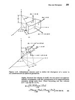
The
electric
field
distribution
due
to
external
sources
is
disturbed
by
the
addition
of
a
conducting
or
dielectric
body

because
the
resulting
induced
charges
also
contribute
to
the
field.
The
complete
solution must
now
also
satisfy
boundary
conditions imposed
by
the
materials.
4-1
THE
UNIQUENESS
THEOREM
Consider
a
linear
dielectric
material

where
the
permittivity
may vary
with
position:
D
=
e(r)E
=
-e(r)VV
(1)
The
special
case
of
different
constant
permittivity
media
separated
by
an
interface
has
e
(r)
as
a
step

function.
Using
(1)
in
Gauss's
law
yields
V
-
[(r)VV]=-pf
(2)
which
reduces
to
Poisson's
equation
in
regions
where
E
(r)
is
a
constant.
Let
us
call
V,
a
solution

to
(2).
The
solution
VL
to
the
homogeneous
equation
V
-
[e(r)V
VI=
0
(3)
which
reduces
to
Laplace's
equation
when
e(r)
is
constant,
can
be
added
to
Vp
and

still
satisfy
(2)
because
(2)
is
linear
in
the
potential:
V
-
[e
(r)V(
Vp
+
VL)]
=
V
[e
(r)V
VP]
+V
[e
(r)V
VL]
=
-Pf
0
(4)

Any
linear
physical
problem
must
only
have
one
solution
yet
(3)
and
thus
(2)
have
many
solutions.
We
need
to
find
what
boundary
conditions
are
necessary
to
uniquely
specify
this

solution.
Our
method
is
to
consider
two
different
solu-
tions
V
1
and
V
2
for the
same
charge
distribution
V
(eV
Vi)=
-P,
V
(eV
V
2
)
=
-Pf

(5)
so
that
we
can
determine
what
boundary
conditions
force
these solutions
to
be
identical,
V,
=
V
2
.
___
Boundary
Value Problems
in
Cartesian
Geometries
259
The
difference
of
these

two
solutions
VT
=
V,
- V
2
obeys
the
homogeneous equation
V*
(eV
Vr)
=
0
(6)
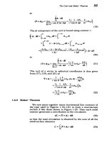
We
examine
the
vector expansion
V
*(eVTVVT)=
VTV
(EVVT)+eVVT"
VVT=
eVVTI
2
(7)
0
noting

that
the
first
term
in
the
expansion
is
zero
from
(6)
and
that
the
second
term
is
never
negative.
We
now
integrate
(7)
over
the
volume of
interest
V,
which
may

be
of
infinite
extent
and
thus
include
all
space
V.
V(eVTVVT)dV=
eVTVVT-dS=
I
EIVVTI
dV
(8)
The
volume
integral
is
converted
to
a
surface
integral
over
the
surface
bounding
the

region
using the
divergence
theorem.
Since
the
integrand
in
the
last
volume
integral
of
(8)
is
never
negative,
the integral
itself can
only
be
zero
if
VT
is
zero
at
every
point
in

the
volume
making the
solution
unique
(VT
=
O0 V
1
=
V2).
To
force
the
volume
integral
to
be zero,
the surface integral
term
in
(8)
must
be zero.
This
requires
that
on
the
surface

S
the
two
solutions
must
have
the
same
value
(VI
=
V2)
or
their
normal
derivatives
must
be
equal
[V
V
1
-
n
=
V
V
2
n].
This

last
condition
is
equivalent
to
requiring
that
the
normal
components
of
the
electric
fields
be
equal
(E
=
-V
V).
Thus,
a
problem
is
uniquely
posed
when
in
addition
to

giving
the
charge
distribution,
the potential
or
the
normal
component
of
the
electric
field
on
the
bounding
surface
sur-
rounding
the
volume
is
specified.
The
bounding
surface
can
be
taken
in

sections
with
some
sections
having
the
potential
specified
and
other
sections
having
the
normal
field
component
specified.
If
a
particular
solution
satisfies
(2)
but
it
does
not
satisfy
the
boundary

conditions, additional
homogeneous
solutions
where
pf
=
0,
must
be
added
so
that
the
boundary
conditions
are
met.
No
matter
how
a
solution
is
obtained,
even
if
guessed,
if
it
satisfies

(2)
and
all
the
boundary
conditions,
it
is
the
only
solution.
4-2
BOUNDARY VALUE PROBLEMS
IN
CARTESIAN
GEOMETRIES
For
most
of
the problems
treated
in
Chapters
2
and
3
we
restricted
ourselves
to

one-dimensional
problems where
the
electric
field
points
in
a single
direction
and
only
depends
on
that
coordinate.
For
many
cases,
the
volume
is
free
of
charge
so
that
the
system
is
described

by
Laplace's
equation. Surface
260
Electric
Field
Boundary
Value Problems
charge
is
present
only
on
interfacial
boundaries
separating
dissimilar
conducting
materials.
We now
consider
such
volume
charge-free
problems
with
two-
and
three
dimen-

sional
variations.
4-2-1
Separation
of
Variables
Let us
assume
that
within
a
region
of
space
of
constant
permittivity
with
no
volume
charge,
that
solutions
do
not
depend
on
the
z
coordinate.

Then
Laplace's
equation
reduces
to
8
2V
O2V
ax2
+y2
=
0
(1)
We
try
a
solution
that
is
a
product
of
a
function
only
of
the
x
coordinate
and

a
function
only
of
y:
V(x,
y)
=
X(x)
Y(y)
(2)
This
assumed solution
is
often convenient
to
use
if
the
system
boundaries
lay
in
constant
x
or
constant
y
planes.
Then

along
a
boundary,
one
of
the functions
in
(2)
is
constant.
When
(2)
is
substituted
into
(1)
we
have
_d'2X
d2Y
1
d2X
1
d2,Y
Y-
+X
=
0
+
(3)

dx
dy
X
dx2
Y
dy
where
the
partial
derivatives
become total
derivatives
because
each
function
only
depends
on
a single
coordinate.
The
second
relation
is
obtained
by
dividing
through
by
XY

so
that
the
first
term
is
only
a
function
of
x
while
the
second
is
only
a
function
of
y.
The
only
way
the
sum
of these
two
terms
can
be

zero
for
all
values
of
x
and
y
is
if
each
term
is
separately
equal
to
a
constant
so
that
(3)
separates into
two
equations,
1 d
2
X
2
1 d
2

Y_k
X
k
d
(4)
where
k
2
is
called
the
separation
constant
and
in
general
can
be
a
complex
number.
These
equations
can
then
be
rewritten
as
the
ordinary

differential
equations:
d
2
X
d
2
Sk-2X=
O,
++k'Y=O2
dx
dy
Boundary
Value
Problems
in
Cartesian
Geometries
261
4-2-2
Zero
Separation
Constant
Solutions
When
the
separation
constant
is
zero

(A
2 =
0)
the
solutions
to
(5)
are
X
=
arx
+bl,
Y=
cry+dl
where
a,,
b
1
,
cl,
and
dl
are
constants.
The
potential
is
given
by
the

product
of these
terms
which
is
of
the
form
V
=
a
2
+
b
2
x
+
C
2
y
+
d
2
xy
The
linear
and
constant
terms
we

have seen
before,
as
the
potential
distribution
within
a
parallel
plate
capacitor
with
no
fringing,
so
that
the
electric
field
is
uniform.
The
last
term
we
have
not
seen
previously.
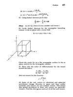
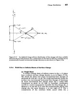
(a)

Hyperbolic
Electrodes
A
hyperbolically
shaped
electrode
whose
surface
shape
obeys
the
equation
xy
=
ab
is
at
potential
Vo
and
is
placed
above
a
grounded
right-angle
corner
as
in
Figure

4-1.
The
Vo
0
5
25
125
Equipotential
lines
-
- -
Vo
ab
Field
lines
-
y2
-
X2
=
const.
Figure
4-1
The
equipotential
and
field
lines
for
a

hyperbolically
shaped
electrode
at
potential
Vo
above
a
right-angle
conducting
corner
are
orthogonal
hyperbolas.
262
Electric
Field
Boundary
Value
Problems
boundary
conditions
are
V(x
=
0)=
0,
V(y
=
0)=

0,
V(xy
=
ab)=
Vo
(8)
so
that
the
solution
can be
obtained
from
(7)
as
V(x,
y)=
Voxy/(ab)
(9)
The
electric
field
is
then
Vo
E
=
-VVV
=
[yi,

+xi,]
(10)
ab
The
field
lines
drawn
in
Figure
4-1
are the
perpendicular
family
of
hyperbolas
to
the
equipotential
hyperbolas
in
(9):
dy
E,
xy
2
-x
2
=
const
(11)

dx
E.
y
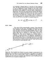
(b)
Resistor
in
an
Open
Box
A
resistive
medium
is
contained
between
two
electrodes,
one
of
which
extends
above
and
is
bent
through
a
right-angle
corner
as

in
Figure
4-2.
We
try zero
separation
constant
Vs
Vr
N\
NN
.
t-

r
-

-
-

E
-
~
- - - -

- - - - - -



M R

&y E,
I
-x
dr
E,
s-y
=
-y
-
)2
-
(X
-
1)2
=
const.
V=O
Depth
w
I
I
>
x
0
I
Figure
4-2
A
resistive
medium

partially
fills
an
open
conducting
box.
SV
V
S
L
-lI-+
=J
Vo
s-d
I
s
Is
0.1
0.2
0.3
0.4
0.5
0.6
0.7
0.8
0.9
v-
V
d
Boundary

Value
Problems
in
Cartesian
Geometries
263
solutions
given
by
(7)
in
each
region
enclosed
by
the
elec-
trodes:
V=
{ai+bix+ciy+dixy
'
oy-•-d
(12)
a
2
+ b
2
x+c
2
y+d

2
xy,
d
y
s
With
the potential
constrained
on
the
electrodes
and
being
continuous
across
the
interface,
the
boundary
conditions
are
V(x=0)=
Vo=aI+cIy
a
= V o,
cl
=0
(O y
Sd)
170

a
+bll+c
ly+d
ly=:bl=-Vo/1,
di=0
V(x
=
1)=
0=
vo
(
y
d)
a2
+
b
2
1+c
2
y+d
2
y
a
2
+ b
2
l
=
0,
C

2
+d
2
1=0
(d
y -
s)
V(y=s)=O=a
2
+b
2
x+c
2
s+d
2
xs
=a
2
+ C
2
s=O,
b
2
+d
2
s=O
70
70
V(y=d+)=
V(y=d-)=ai+bilx+c

d+
di
xd
=a
2
+ b
2
x
+
C2d
+ d
2
xd
(13)
>al=
Vo=a
2
+c
2
d,
b
=
-V/l=b
2
+d
2
d
so
that
the constants

in
(12)
are
a=
Vo,
b=-
Vo/1l,
cl=0,
dl=0
Vo Vo
a
2
,
b2
-
(14)
(I
-
d/s)
b
(1 -
d/s)'
V
0
V
0
C2
=
d
2

-
s(1
-d/s)'
Is(1
-d/s)
The
potential
of
(12)
is
then
Vo(1
-
x/1),
O-
y!
-d
V=
o( +
(15)
V- I
-+-)
,
d:yss
s
s-d
l
s
Is'
with

associated
electric
field
Vo.
-
ix,
Oysd
E=
-V
V=|
(16)
s )
I
+
1
)
]
,
d<y<s
Note
that
in
the
dc
steady state,
the
conservation
of
charge
boundary

condition
of
Section
3-3-5
requires
that
no
current
cross
the interfaces
at
y
=
0
and
y
=
d
because
of
the
surround-
ing
zero
conductivity
regions.
The current
and,
thus,
the

264
Electric
Field Boundary
Value Problems
electric
field
within
the
resistive
medium
must
be
purely
tangential
to
the
interfaces,
E,(y
=
d)=E,(y
=0+)=0.
The
surface
charge
density on
the
interface
at
y
=

d
is
then
due
only
to
the
normal
electric
field
above,
as
below,
the
field
is
purely
tangential:
of(y=d)=EoE,(y=d+)-CE,
(y=d_)=
_
•
1
(17)
The
interfacial
shear
force
is
then

S•EoVO
F=
oEx(yd)wdx=

w
(18)
0
2(s
-
d)
If
the
resistive
material
is
liquid,
this
shear
force
can
be used
to
pump
the
fluid.*
4-2-3
Nonzero
Separation
Constant
Solutions

Further
solutions
to
(5)
with
nonzero
separation
constant
(k
2
#
0)
are
X
=
Al
sinh
kx
+A
2
cosh
kx
=
B1
ekx
+ B
2
e-kx
Y=
C,

sin
ky
+ C
2
cOs
ky
=
Dl
eik
+D
2
e
- k
y
(19)
When
k
is
real,
the
solutions
of
X
are
hyperbolic
or
equivalently
exponential,
as
drawn

in
Figure
4-3,
while
those
of
Y
are
trigonometric.
If
k
is
pure
imaginary,
then
X
becomes
trigonometric
and
Y
is
hyperbolic
(or
exponential).
The
solution
to
the
potential
is

then
given
by
the
product
of X
and
Y:
V
=
El
sin
ky
sinh
kx
+ E
2
sin
ky
cosh
kx
(20)
+E
3
cos
ky
sinh
kx
+ E
4

cos
ky
cosh
kx
or
equivalently
V
=
F
1
sin
ky
e
kx
+ F
2
sin
ky
e
-
Ax
+ F
3
cos
ky
e
k
x
+ F
4

cos
ky
e-'x
(21)
We
can
always
add the
solutions
of
(7)
or
any
other
Laplacian
solutions
to
(20)
and
(21)
to
obtain
a
more
general
*
See
J. R.
Melcher
and

G.
I.
Taylor,
Electrohydrodynamics:
A
Review
of
the
Role
of
Interfacial
Shear
Stresses,
Annual
Rev.
Fluid
Mech.,
Vol.
1,
Annual
Reviews,
Inc.,
Palo
Alto,
Calif.,
1969,
ed.
by
Sears
and

Van
Dyke,
pp.
111-146.
See
also
J. R. Melcher,
"Electric
Fields
and Moving Media",
film
produced
for
the
National
Committee
on
Electrical
Engineering
Films
by
the
Educational
Development
Center,
39
Chapel
St.,
Newton, Mass.
02160.

This
film
is
described
in
IEEE
Trans.
Education
E-17,
(1974)
pp.
100-110.
I~
I
__