Electromagnetic Field Theory: A Problem Solving Approach Part 31 ppt

Separation
of
Variables
in
Cylindrical
Geometry
275
The
other
time-dependent
amplitudes
A
(t)
and
C(t)
are
found
from
the
following
additional
boundary
conditions:
(i)
the
potential
is
continuous
at
r
=

a,
which
is
the
same
as
requiring
continuity
of
the
tangential
component
of
E:
V(r=
a.)=
V(r
=
a-)
E6(r
=
a-)
=
E#(r
=
a+)
Aa
=
Ba
+

Cia
(17)
(ii)
charge
must
be
conserved
on
the interface:
Jr(r
=
a+)
-,(r
=
a_)+
=
0
at
S>a,
Er(r
=
a+)
-
0-
2
E,(r
=
a-)
+-a
[eIE,(r

=
a+)-
e
2
Er(r
=
a-)]
=
0
(18)
In
the
steady state,
(18)
reduces
to
(11)
for
the
continuity
of
normal
current,
while
for
t=
0
the
time
derivative

must
be
noninfinite
so
of
is
continuous
and
thus
zero
as
given
by
(10).
Using
(17)
in
(18)
we
obtain
a
single
equation
in
C(t):
d-+
+
2
C
-a

(Eo(
0"
2
)+(eI-
2
)
dt
61+E2
dt
(19)
Since
Eo
is
a
step
function
in
time,
the
last
term
on
the
right-hand
side
is
an impulse
function,
which
imposes

the
initial
condition
2 (8 - E82)
C(t
=
0)
=
-a
Eo
(20)
so
that
the
total
solution
to
(19)
is
2/0.1
(-0
2(0.182-0.281)
-
1
A,
81
82
C(t)=
aEo
-

+
,2(
-0
7=
\l+0.2
(o0+0o2-)
(1+E2)
r0l
+0"2
(21)
The
interfacial
surface
charge
is
o0f(r
=
a, t)
=
e
IEr(r
=
a+) - E
2
E,(r
=
a-)
=
-e,(B
-)'+

2
A]
cos
4
[(6-E2)Eo+(E,
+E)
-2]
cos4
2(0281-0.82
)
2(
-
)
Eo[1-e
-
]
cos
4
(22)
0.1
+
0.2
276
Electric
Field
Boundary
Value
Problems
The
upper

part
of
the
cylinder
(-r/2
047
r/2)
is
charged
of
one
sign while
the
lower
half
(7r/2:5
46
r)
is
charged
with
the
opposite
sign,
the net
charge
on
the
cylinder
being

zero.
The
cylinder
is
uncharged
at each
point
on
its
surface
if
the
relaxation
times
in
each
medium
are
the
same,
E
1
/o'
1
=
e2/0r2
The
solution
for
the

electric
field
at
t
=
0
is
2Eo
2e
1
Eo.
[cos
[Sir-
sin
4i0]
=
i.,
r<a
61+62
E1+62
a
8
2
-81
t=0)=
+
E0
+a
2+
2)

COS
,ir
(23)
[
a
82r81662
-1
)
-
sin
4,i
6
],
r>a
61r
+E2
The
field
inside
the
cylinder
is
in
the
same
direction
as
the
applied
field,

and
is
reduced
in
amplitude
if
62>81
and
increased
in
amplitude
if
e2
<
El,
up
to
a
limiting factor
of
two
as
e1
becomes
large
compared
to
e2.
If
2

=
E1,
the
solution
reduces
to
the
uniform
applied
field
everywhere.
The
dc
steady-state
solution
is
identical
in
form
to
(23)
if
we
replace the
permittivities
in
each
region
by
their

conduc-
tivities;
2o.E
o
20.Eo
0
[cosi,r-
sin4i
21~
i.,
r<a
al1
+
2
71
+ 02
2
Ft
a
02-01
,
E(t
-
co)
= Eo
0
•+
0
cos
ir

(24)
'r
1+or2)
-(1
aI
'2-rln
>in.,
r>a
(b)
Field
Line
Plotting
Because
the region
outside
the
cylinder
is
charge
free,
we
know
that
V
E
=0.
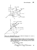
From
the
identity
derived

in
Section
1-5-4b,
that
the
divergence
of
the curl
of
a
vector
is
zero,
we
thus
know
that
the
polar
electric
field
with
no
z
component
can be
expressed
in
the
form

E(r,
4)
=
VX
(r,
4,)i.
I
a.
ax.
i, 14
(25)
ra46
ar
where
x
is
called
the stream function.
Note
that
the stream
function
vector
is
in
the
direction
perpendicular
to
the

elec-
tric
field
so
that
its
curl
has
components
in
the
same
direction
as
the
field.
Separation
of
Variables
in
Cylindrical
Geometry
277
Along
a
field
line,
which
is
always

perpendicular
to
the
equipotential
lines,
dr
E, 1
/
(26)
r
d4
Es
r
a8/8r
By
cross
multiplying
and grouping
terms
on
one
side
of
the
equation,
(26)
reduces
to
d.
= dr+-d

4
=
0>Y
=
const
(27)
ar
a84
Field
lines
are
thus
lines
of
constant
1.
For the
steady-state
solution of
(24),
outside
the
cylinder
1
a1
/
a2
o-
o*tI
Iay

E=
rEoI
1+
)
cos
rrr
o
+
o
(28)
2
-ý=E.s=
-Eo
1
2I-
sin
ar
r2
+
0o2
we
find
by
integration
that
I
=
Eo(r+
a-
t

Ti
sin
(29)
r
or
+
C'2)
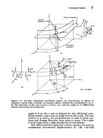
The
steady-state'field
and
equipotential
lines
are
drawn
in
Figure
4-8
when
the
cylinder
is
perfectly
conducting
(o
2
->
ox)
or
perfectly
insulating

(or
2
=
0).
If
the
cylinder
is
highly
conducting,
the
internal
electric
field
is
zero
with
the
external
electric
field
incident
radially,
as
drawn
in
Figure
4-8a.
In contrast,
when

the
cylinder
is
per-
fectly
insulating, the
external
field
lines
must
be
purely
tangential
to
the
cylinder
as
the incident
normal
current
is
zero,
and
the
internal
electric
field
has
double
the

strength
of
the applied
field,
as
drawn
in
Figure
4-8b.
4-3-3
Three-Dimensional
Solutions
If
the
electric
potential
depends
on
all
three
coordinates,
we
try
a
product
solution
of
the
form
V(r,

4,
z)
=
R(r)4(d)Z(z)
(30)
which
when
substituted
into
Laplace's
equation
yields
ZD
d
d
RZd
2
4+
d
2
Z
(31)
•rr
+
2
+
R - -
= 0
(31)
r

-dr dr
r
d0
Z
We
now
have
a
difficulty,
as
we
cannot
divide
through
by
a
factor
to make each
term
a
function
only
of
a
single
variable.
278
Electric
Field
Boundary

Value
Problems
2
1 AL1
r a
V/(Eoa)
Eoi,
=
Eo(Jr
coso-
i¢,
sing)
Figure
4-8
Steady-state
field
and equipotential
lines
about
a
(a)
perfectly
conducting
or
(b)
perfectly
insulating
cylinder
in
a

uniform
electric
field.
However,
by
dividing
through
by
V
=
RDZ,
Sd
d
d
I
d
2
4
1 d
2
Z
Rr
dr
ýr
r2
d•
d
Z
=
0

-k
k
2
we
see
that
the
first
two
terms
are
functions
of
r
and
4
while
the
last
term
is
only
a
function
of
z.
This
last
term
must

therefore
equal
a
constant:
2.9
(Alsinhkz+A
2
coshkz,
kO0
I
dZ
Z
=
Z
dz
Z+A,
A~zz+A4,
k=0
-*C~ · L ^-
r>a
r<a
2
a
f_
Separation
of
Variables
in
Cylindrical
Geometry

-2Eorcoso
r<a
-Eoa(a
+
)cosO
r>a
2Eo
(cosi,
-
sin
iO)
=
2E
o
i,
E=-VV
Eo
a
2
a
2
E(1
2
)cosi,
-(1+
r
2
)sinoiJ
r r
279

r<a
r>a
Eoa
-4.25
3.33
-2.5
-2.0
1.0
-0.5
0.0
0.5
1.0
2.0
2.5
3.33
a
2
a
2
coto
(1+ )
( -
a)sine
=
const
a
r
Figure
4-8b
The

first
two
terms
in
(32)
must
now
sum
to
-k
2
so
that
after
multiplying
through
by
r
2
we
have
rd
dR
22
1d
2
D
R
dr r+k
r

+-
=0
Now
again
the
first
two
terms
are
only
a
function
of
r,
while
the
last
term
is
only
a
function
of
0
so
that
(34)
again
separates:
rd

r
+k2r
2
2
Rdr
dr
r
1
d
2
2
d2-n
to•i•
=
Edl
cos
-
Isln
o)
ZU0
Electric
FieldBoundary
Value Problems
where
n
2
is
the
second
separation

constant.
The
angular
dependence
thus
has
the
same
solutions
as
for
the
two-
dimensional
case
(B,
sinn
+h
B
Rco'
nd
n
0
B, Ds n
,03(
D
D4,
n
ý
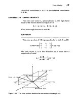
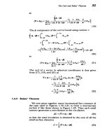
The

resulting
differential
equation for
the
radial
dependence
d
dR\
r-
r-
+
(k
2
-n2)R
=
0
ar
\
ar/
is
Bessel's
equation
and
for nonzero
k
has
solutions
in
terms
(a)

Figure
4-9
The
Bessel
functions
(a)
J.(x)
and
I.(x),
and
(b)
Y.(x)
and
K.
(x).
&'I
t•
tA
1
x
Separation
of
Variables
in
Cylindrical
Geometry
281
of
tabulated functions:
C]J,(kr)+CY,,(kr),

k
•0
R=
C
3
rn
+ C
4
r
-
,
k=
0,
n
0
(38)
C
5
In
r+
C
6
,
k=0, n=0
where
J.,
is
called
a
Bessel

function
of
the
first
kind
of
order
n
and
Y.
is
called
the
nth-order
Bessel
function
of
the
second
kind.
When
n
=
0,
the
Bessel
functions
are
of zero
order

while
if
k
=
0
the
solutions
reduce
to
the
two-dimensional
solutions
of
(9).
Some
of
the
properties
and
limiting
values
of
the
Bessel
functions
are illustrated
in
Figure
4-9.
Remember

that
k
2.0
1.5
1.0
0.5
0.5
1.0
Figure
4-9b
282
Electric
Field
Boundary
Value
Problems
can
also
be
purely
imaginary
as
well
as
real.
When
k
is
real
so

that
the
z
dependence
is
hyperbolic
or
equivalently
exponen-
tial,
the
Bessel
functions
are
oscillatory
while
if
k
is
imaginary
so
that
the
axial
dependence
on
z
is
trigonometric,
it

is
con-
venient
to
define
the
nonoscillatory modified
Bessel
functions
as
I.(kr)=
j"J.(fkr)
(39)
K,(kr)
=
ji
j "
+
U[(jkr)
+jY(ikr)]
As
in
rectangular
coordinates,
if
the
solution
to
Laplace's
equation

decays
in
one
direction,
it
is
oscillatory
in
the
perpendicular
direction.
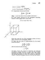
4-3-4
High
Voltage
Insulator
Bushing
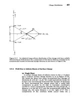
The
high
voltage
insulator
shown
in
Figure
4-10 consists
of
a
cylindrical disk
with
Ohmic
conductivity

or
supported
by
a
perfectly
conducting
cylindrical
post
above
a
ground
plane.*
The
plane
at
z =
0
and
the
post
at
r
=
a
are
at
zero
potential,
while
a

constant potential
is
imposed
along the
circumference
of
the
disk
at
r
=
b.
The
region
below
the
disk
is
free
space
so
that
no
current
can cross
the
surfaces at
z
=
L

and
z
=
L
-
d.
Because
the
boundaries
lie
along
surfaces at
constant
z
or
constant
r
we
try
the
simple
zero
separation constant
solutions
in
(33)
and
(38),
which
are

independent
of angle
4:
V(r,z)
=Az+Blz
lnr+Cllnr+D
1
,
L-d<z<L
A
2
z+B
2
zlnr+C21nr+D
2
,
O-z<L-d
(40)
Applying
the
boundary
conditions
we
relate
the
coefficients
as
V(z
=
0)

=
0
C
= D
2
=
0
(A
2
+B
2
In
a
= 0
V(r=a)=0>
A
1
+Bllna=0
(C
1
In a
+DI
= 0
V(r=b,r>L-d)-Vo•(
C1lnb+D1
= V o
V(z
=
(L
-

d)-)
=
V(z
=
(L
-
d)+)
(L
-
d)
(A
+ B
2
In
r)
=(L-d)(A,+B
Iln
r)+
C
lnr+Dj
*
M.
N.
Horenstein,
"Particle
Contamination
of
High
Voltage
DC

Insulators,"
PhD
thesis,
Massachusetts
Institute
of
Technology,
1978.
I
___
Separation
of
Variables
in
Cylindrical
Geometry
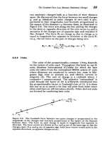
r=b
Field lines
2
= r
2
[ln(r/a)
-1]
+
const
2

Equipotential
V
Vosln(r/a)

V-
lines
(L

d)In(b/a)
(b)
Figure
4-10
(a) A
finitely
conducting
disk
is
mounted
upon
a
perfectly
conducting
cylindrical
post
and
is
placed
on
a
perfectly
conducting
ground
plane.
(b)

Field
and
equipotential
lines.
283
L-
V
=
V
0
a-•
o
Electric
Field
Boundary
Value Problems
Vo
In
(bla)'
which
yields
the
values
Al=
B
1
=
0,
(L
-dVo

In
(/a)
(L
-d)
In
(b/a)
The
potential of
(40)
is
then
Vo
In
(r/a)
In
(b/a)
'
V(r,
z)
=
In
(a)
Voz
In
(r/a)
w(L
-
d)
In
(b/a)

with
associated
electric
field
Vo
r
In
(bla)
r
E=
-VV=
-
d
(In
ri,+
(L
-d)
In
(bla)
a
r
Vo
In
a
D=
(42
In
(b/a)
(42)
C

2
= D
2
=
0
L-dszsL
OzSL-d
L-d<z<L
(44)
O<z<L-d
The
field
lines
in
the
free
space
region
are
dr
=
Er
z
rn
1+const
dz
E,
rl
In
(rla)

a
2J
(45)
and
are
plotted
with
the
equipotential
lines
in
Figure
4-10b.
4-4
PRODUCT
SOLUTIONS
IN
SPHERICAL
GEOMETRY
In
spherical
coordinates,
Laplace's
equation
is
a1
2
a
V
1

a
/sin
1 a
2
v
rr\
r
2
2
sin
0 0
sin•
0
,
4-4-1
One-Dimensional
Solutions
If
the
solution
only
depends
on
a
single spatial
coordinate,
the
governing
equations
and

solutions
for
each
of
the
three
coordinates
are
d
/
dV(r)\
A,
dr
dr
/
r
284
Vo
B
2
=
(L
-d)
In
(b/a)'
_I~_
~__··
(i)
-
r'

r=0=
V(r)=-+A2