Electromagnetic Field Theory: A Problem Solving Approach Part 32 docx

Product
Solutions
in
Spherical
Geometry
285
(ii)
d
sin
0
=
0
V(0)=B
1
In
tan
+B
2
(3)
d
2
V(O)
(iii)
d
=
0
V()
=
CIO
+
C2

(4)
We
recognize
the
radially
dependent
solution
as
the
poten-
tial
due
to
a
point
charge.
The
new
solutions
are
those
which
only
depend
on
0
or
4.
EXAMPLE
4-2

TWO
CONES
Two
identical
cones
with
surfaces at
angles
0
=
a
and
0
=
ir-a
and
with
vertices
meeting
at
the
origin, are
at
a
poten-
tial
difference
v,
as
shown

in
Figure
4-11.
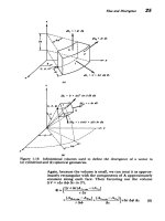
Find
the potential
and
electric
field.
1
0
In(tan
)
2
In
(tan
)
2rsinO
In(tan
)
/2
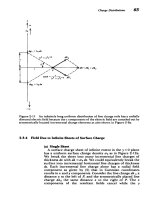
Figure
4-11
Two
cones
with vertices
meeting
at
the
origin
are

at
a
potential
difference
v.
i
286
Electric
Field
BQundary
Value
Problems
SOLUTION
Because
the
boundaries
are
at
constant
values
of
0,
we
try
(3)
as
a
solution:
V()
=

Bl
In
[tan
(0/2)1+
B
2
From
the
boundary
conditions
we
have
v(o
=
a)
=v
2
-v v
V(O
=
r
-a)=
-
Bl=
B2=0
2
2
In
[tan
(a/2)]'

B
so
that
the
potential
is
v=
In
[tan
(0/2)]
V(0)
=
2
In
[tan
(a/2)]
with
electric
field
-v
E=
-VV=
is
2r
sin
0
In
[tan
(a/2)]
4-4-2

Axisymmetric
Solutions
If
the
solution
has
no
dependence
on the
coordinate
4,
we
try
a
product
solution
V(r,
0)
=
R(r)O(0)
(5)
which
when
substituted
into
(1),
after
multiplying
through
by

r
2
/RO,
yields
I
d
2
dR'
d
dO
_r
+ .+sin
0
( -s =
0
(6)
Rdr
dr
sin
0
dO
Because
each
term
is
again
only
a
function
of

a
single
vari-
able,
each
term
is
equal to
a
constant.
Anticipating
the
form
of
the
solution,
we
choose
the separation
constant
as
n(n
+
1)
so
that
(6)
separates
to
r r'

-
-n(n+1)R=0
(7)
di
d\
-I
sin
-,
+n(n
+ 1)
sin
9=0
au
adO
I-
Product
Solutions
in
Spherical
Geometry
287
For
the
radial
dependence
we
try
a
power-law
solution

R
=
Arp
(9)
which
when
substituted
back
into
(7)
requires
p(p
+ 1)
=
n(n
+ 1)
(10)
which
has
the
two
solutions
p=n,
p
=
-(n+1)
(11)
When n
=
0

we
re-obtain
the
l/r
dependence
due
to
a
point
charge.
To
solve
(8)
for
the
0
dependence
it
is
convenient
to
intro-
duce
the
change
of
variable
i =
cos
0

(12)
so
that
de
dedp
de
Ode
d-sin
=
_-(1 /
2
Pd)
(13)
dO
d1
dO
dp
dp
Then
(8)
becomes
d
2
de
-±
(p-2
)d-
+n(n+1)O=0
(14)
which

is
known
as
Legendre's
equation.
When
n
is
an
integer,
the
solutions
are
written
in
terms of
new
functions:
e
=
B.P,,()+
C.Q,(P)
(15)
where
the
P.(i)
are
called
Legendre
polynomials

of
the
first
kind
and
are
tabulated
in
Table
4-1.
The
Q.
solutions
are
called
the
Legendre
functions of
the
second
kind
for
which
the
first
few
are
also
tabulated
in

Table
4-1.
Since
all
the
Qn
are
singular
at
0
= 0
and
9
=
ir,
where
P
=
* 1,
for
all
problems
which
include
these
values
of
angle,
the
coeffcients

C.
in
(15)
must
be zero,
so
that
many
problems
only
involve
the
Legen-
dre
polynomials
of
first
kind,
P.(cos
0).
Then
using
(9)-(11)
and
(15)
in
(5),
the
general
solution

for the
potential
with
no
*
dependence
can
be
written
as
V(r,
0)=
Y
(A.r"
+
Br-"+I))P.(cos
0)
(16)
n-O
Electric
Field
Boundary
Value
Problems
Table
4-1
Legendre
polynomials
of
first

and
second
kind
n
P.(6
=
cos
0)
0
1
1
i
=
cos
0
2
(30
2
-
1)
=
(3
Cos
2
0
-
1)
Q.(-
=
cos

0)
, (1+0
PIn
-( /
(32
()
+P
3
()~-
20
3
((50S-
S3)
=
-
(5
cos
s
0
-
3
cos
0)
1
d"'
m
d
(p2-
1)m
2"m!

dp"
4-4-3
Conducting
Sphere
in
a
Uniform
Field
(a)
Field Solution
A
sphere
of
radius
R,
permittivity
E
2
,
and
Ohmic
conduc-
tivity
a
2
is
placed
within
a
medium

of
permittivity
el
and
conductivity
o-1.
A
uniform
dc
electric
field
Eoi.
is
applied
at
infinity.
Although
the
general
solution
of
(16)
requires
an
infinite
number
of terms,
the
form
of

the
uniform
field
at
infinity in
spherical
coordinates,
E(r
-*
co)
= Eoi.
=
Eo(i,
cos
0
-
ie
sin
0)
suggests
that
all
the
boundary
conditions
can
be
met
with
just

the
n
=
1
solution:
V(r,
0)
=Ar
cos
0,
rsR
V(Br+C/r
2
)
cos
0,
r-R
We
do not
include
the
l/r
2
solution
within
the sphere
(r
<
R)
as

the
potential
must
remain
finite
at
r
= 0.
The
associated
288
I
Product
Solutions
in
Spherical
Geometry
289
electric
field
is
E=-VV=
-A(ir
cos
0-ie
sin
0)=
-Ai,,
r<R
-(B

-2C/r
3
)
cos
Oi+(B
+C/r
)
sin
0i.,
r>R
(19)
The
electric
field
within
the
sphere
is
uniform
and
z
direct-
ed
while
the solution
outside
is
composed
of
the

uniform
z-directed
field,
for
as
r
oo
the
field
must
approach
(17)
so
that
B
=
-Eo
0
,
plus
the
field
due
to
a
point
dipole
at
the
origin,

with
dipole
moment
Pý
=
41re
C
(20)
Additional
steady-state
boundary
conditions
are
the
continuity
of
the
potential
at
r
=
R
[equivalent
to
continuity
of
tangential
E(r
=R)],
and

continuity
of
normal
current
at
r
=
R,
V(r
=
R)=
V(r
=
R-)> Ee(r
=
R+)=
Eo(r
=
R_)
>AR
=
BR
+
C/R
2
,(r
=
R+)
=],(r
=

R-)zoriEr,(r=
R+)
=
r
2
E,(r
=
R)
(21)
>ral(B
-2C/R
s)
=
or
2
A
for
which
solutions
are
3o'
(2'a-
l)RS
A
=
Eo,
B =
-Eo,
C =
Eo

(22)
2orl
+
a-
2
2ol
+ o
The
electric
field
of
(19)
is
then
3So-Eo
3Eo
1
E
.
(i,
cos
0 -
ie
sin
0)=
i,,
r<R
2a0
1
+

2
2a,
+
o,2
E=
Eo
1+
2
R
a-2
)
cos
Oi,
(23)
(
R3
(0-oin)
6si
,
r>R
rs(2cri
+
0'2))
s r
The
interfacial
surface
charge
is
orf(r

=
R)
=
eiE,(r
=
R+)-
E
2
E(r
=
R-)
3(o2E
1-
oIE2)Eo
c
1
os
0
(24)
2crl
+
02
which
is
of
one
sign
on
the
upper

part
of
the
sphere
and
of
opposite
sign
on
the
lower
half
of
the
sphere.
The
total
charge
on
the
entire
sphere
is
zero.
The
charge
is
zero
at
290

Electric
Field
Boundary
Value Problems
every
point
on
the
sphere
if
the
relaxation
times
in
each
region
are
equal:
(25)
O"
I
'2
The
solution
if
both
regions
were
lossless
dielectrics

with
no
interfacial
surface
charge,
is
similar
in
form
to
(23)
if
we
replace
the
conductivities
by
their
respective
permittivities.
(b)
Field
Line
Plotting
As
we
saw
in
Section
4-3-2b

for
a
cylindrical
geometry,
the
electric
field in
a
volume
charge-free
region
has
no
diver-
gence,
so
that
it
can
be
expressed
as
the
curl
of
a
vector.
For
an
axisymmetric

field in
spherical
coordinates
we
write
the
electric
field
as
-
((r,
0).
E(r,
0)=
VX
rsin
1
al
1
a1.
=
2,
is
(26)
r
sin
0
ao
r
sin

0
ar
Note
again,
that for
a
two-dimensional
electric
field,
the
stream
function
vector
points
in
the
direction
orthogonal
to
both
field
components
so
that
its
curl
has
components
in
the

same
direction
as
the
field.
The
stream
function
I
is
divided
by
r
sin
0
so
that
the
partial
derivatives
in
(26)
only
operate
on
The
field
lines
are
tangent

to
the
electric
field
dr
E
1
ala
(27)
(27)
r
dO
Es
r
allar
which
after
cross
multiplication
yields
d
=
-dr+
dO
=
0
=
const
(28)
ar

O0
so
that
again
I
is
constant
along
a
field
line.
For
the
solution
of
(23)
outside the
sphere,
we
relate
the
field
components
to
the
stream
function using
(26)
as
1

a8
2R(
"______l)_
E,=
= Eo
1
-
cos0
r'
sin
80
a
r
(2a
1
i
+
2
) )
(29)
E
1 =
-Eo
1 -
sin
0
r
sin
0
ar

rs(20
+
2))
Poduct
Solutions
in
Spherical
Geometry
291
so
that
by
integration
the
stream
function
is
r
RS'-
2
'l)
I=
Eo
+)
sin2
0
(30)
2
r(2ao
+0r2)

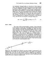
The
steady-state
field
and equipotential
lines
are
drawn
in
Figure 4-12
when
the
sphere
is
perfectly
insulating
(ar
2
=
0) or
perfectly
conducting
(o-2
-0).
-
EorcosO
r<R
R
2r
E•[O-•i-]cos0
rcos2

•
Eo
i,
cosO
i
o
sin0l=
Efoil
r<R
E=-VV=
1
R
3
En
Eo[(1
-
)cosir (1
+
)
sin~i.
r>R
(1
dr
Er
rdO
-
E.
rI
2rV
E

o R
-
-4.0

-3.1

2.1
-1.6

1.3

1.1

0.4

0.0


0.4

-
0.75
1.1

1.3

2.1

3.1

4.0
Eoi,
=
Eo(ircosO - i,
sinO)
(a)
Figure
4-12
Steady-state
field
and
equipotential
lines
about
a (a)
perfectly
insulating
or
(b)
perfectly
conducting
sphere
in
a
uniform
electric
field.


292

Electric
Field
Boundary
Value
Problems
V=
r R
EoR(
-
R
r
2
)cos60
t
Rr2
-VV=
2R3
)C
R
3
o0ir
-(1
_- )
sin0i
0
]
r>
R
(1 + 2
dr

E,
_
r
3
cot
rdO
E
(1
-
.)
P
3
[+
I
5
(
)
2
]sin
2
R
-2.75
- 1.0

-0.6

0.25
0
0.25
0.6

1.0
S
1.75
2.75
Eoi
,
=
Eo(ircosO
-
i0
sin0)
Figure
4-12b
If
the
conductivity
of
the
sphere
is
less
than
that
of
the
surrounding
medium
(O'2<UO),
the
electric

field
within
the
sphere
is
larger
than
the applied
field.
The
opposite
is
true
for
(U
2
>oj).
For
the
insulating
sphere
in
Figure
4-12a, the
field
lines
go
around
the
sphere

as
no
current
can
pass
through.
For
the
conducting sphere
in
Figure
4-12b,
the
electric
field
lines
must
be
incident
perpendicularly.
This
case
is
used
as
a
polarization
model,
for
as

we
see
from
(23)
with 2
-:
oo,
the
external
field
is
the
imposed
field
plus
the
field
of
a
point
r<R
r>R
r
ýi
Product
Solutions
in
Spherical
Geometry
293

dipole
with
moment,
p,
=
4E
i
R
3Eo
(31)
If
a
dielectric
is
modeled
as
a
dilute
suspension
of
nonin-
teracting,
perfectly
conducting spheres
in
free
space
with
number
density

N,
the
dielectric
constant
is
eoEo
+
P
eoEo
+
Np,
e
=
-
=
o(1
+4rR
3N)
(32)
Eo
Eo
4-4-4
Charged
Particle
Precipitation
Onto
a
Sphere
The
solution

for
a
perfectly
conducting
sphere
surrounded
by
free
space
in
a
uniform
electric
field
has
been
used
as
a
model
for
the
charging
of
rain
drops.*
This
same
model
has

also
been
applied
to
a
new
type
of
electrostatic
precipitator
where
small
charged
particulates are
collected
on
larger
spheres.t
Then,
in
addition
to
the
uniform
field
Eoi,
applied
at
infinity,
a

uniform
flux
of
charged particulate
with
charge
density
po,
which
we
take
to
be
positive,
is
also
injected,
which
travels
along
the
field
lines
with
mobility
A.
Those
field
lines
that

start
at
infinity
where
the charge
is
injected
and
that
approach
the
sphere
with
negative
radial
electric
field,
deposit
charged particulate,
as
in
Figure
4-13.
The
charge
then
redistributes
itself
uniformly
on

the
equipotential
sur-
face
so
that
the
total
charge
on
the
sphere
increases
with
time.
Those
field
lines
that
do
not
intersect the
sphere
or
those
that
start
on
the
sphere

do
not
deposit
any
charge.
We
assume
that
the
self-field
due
to
the
injected
charge
is
very
much
less
than
the applied
field
E
0
.
Then
the
solution
of
(23)

with
Ov2
=
00
iS
correct
here,
with
the
addition
of
the
radial
field
of
a
uniformly charged
sphere
with
total
charge
Q(t):
2R3
Q3
E=
[Eo(1+
3)
cos
+ i2]
i

-Eo(1-
)3sin
io,
r 4
7r
rr
r>R
(33)
Charge
only
impacts
the
sphere
where
E,(r
=
R)
is
nega-
tive:
E,(r
=
R)=
3Eo
cos
+
2<0
(34)
47TER
*

See:
F. J.
W.
Whipple
and
J.
A.
Chalmers,
On
Wilson's
Theory
of
the
Collection
of
Charge
by
Falling
Drops,
Quart.
J.
Roy.
Met.
Soc.
70,
(1944),
p.
103.
t
See:

H.
J.
White,
Industrial
Electrostatic
Precipitation
Addison-Wesley,
Reading.
Mass.
1963,
pp.
126-137.
n
+ 1.0
Q.
(a)
Figure
4-13
continuous
positive
[E,(R)<
0]
deposit
charge,
the
field
lines
some
of
the

incident
collection
decreases
as
angular
window
and
y,
11Z
f.
FZ
tz
ano mo1ol1ty P
n
T
E
0
iz
S=

7071
=
0
=
.7071
=
OQ,
Q,
Q.
Q.

(b)
(c)
(d)
(e)
RO
1
2[
1 2
20-
COS
E([+
sin2
0-
=
constant
R
41re
Electric
field
lines
around
a
uniformly
charged
perfectly
conducting
sphere
in
a
uniform

electric
field
with
charge
injection
from
z
=
-ao.
Only
those
field
lines
that
impact
on
the
sphere
with
the
electric
field
radially
inward
charge.
(a)
If
the
total
charge

on
the sphere
starts
out
as
negative
charge
with
magnitude
greater
or
equal
to
the
critical
within
the
distance
y.
of
the
z
axis
impact
over
the
entire
sphere.
(b)-(d)
As

the
sphere
charges
up
it
tends
to
repel
charge
and
only
part
of
the
sphere
collects
charge.
With
increasing charge
the
angular
window
for
charge
does
y,.
(e)
For
Q
-

Q,
no
further
charge
collects
on
the
sphere
so
that
the
charge
remains constant
thereafter. The
have
shrunk
to zero.