3D Graphics with OpenGL ES and M3G- P12 pps

94 LOW-LEVEL RENDERING CHAPTER 3
both depth fail and pass). A very advanced use case for stenciling is volumetric shadow
casting [Hei91].
Depth test
Depth testing is used for hidden surface removal: the depth value of the incoming frag-
ment is compared against the one already stored at the pixel, and if the comparison
fails, the fragment is discarded. If the comparison function is LESS only fragments with
smaller depth value than already in the depth buffer pass; other fragments are discarded.
This can be seen in Figure 3.2, where the translucent object is clipped to the depth values
wr itten by the opaque object. The passed fragments continue along the pipeline and are
eventually committed to the frame buffer.
There are other ways of determining the visibility. Conceptually the simplest approach is
the painter’s algorithm, which sorts the objects into a back-to-front order from the camera,
and renders them so that a closer object always draws over the previous, farther objects.
There are several drawbacks to this. The sorting may require significant extra time and
space, particularly if there are a lot of objects in the scene. Moreover, sorting the prim-
itives simply does not work when the primitives interpenetrate, that is, a triangle pokes
through another. If you instead sort on a per-pixel basis using the depth buffer, visibility
is always resolved correctly, the storage requirements are fixed, and the running time is
proportional to the screen resolution rather than the number of objects.
With depth buffer ing it may make sense to have at least a partial front-to-back rendering
order, the opposite that is needed without a depth buffer. This way most fragments that
are behind other objects will be discarded by the depth test, avoiding a lot of useless frame
buffer updates. At least blending and writing to the frame buffer can be avoided, but
some engines even perform texture mapping and fogging only after they detect that the
fragment survives the depth test.
Depth offset
As already discussed in Section 2.5.1, the depth buffer has only a finite resolution. Deter-
mining the correct depth ordering for objects that are close to each other but not close to
the near frustum plane may not always be easy, and may result in z-fighting, as shown in
Figure 2.11. Let us examine why this happens.

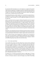
Figure 3.22 shows a situation where two surfaces are close to each other, and how the
distance between them along the viewing direction increases with the slope or slant of the
surfaces. Let us interpret the small squares as pixel extents (in the horizontal direction as
one unit of screen x, in the vertical direction as one unit of depth buffer z), and study the
image more carefully. On the left, no matter where on the pixel we sample the surfaces, the
lower surface always has a higher depth value, but at this z-resolution and at this particular
depth, both will have the same quantized depth value. In the middle image, if the lower
surface is sampled at the left end of the pixel and the higher surface at the right end, they
SECTION 3.5 PER-FRAGMENT OPERATIONS 95
z
x
z
x
z
x
Figure 3.22: The slope needs to be taken into account with polygon offset. The two lines are two
surfaces close to each other, the arrow shows the viewing direction, and the coordinate axes illustrate
x and z axis orientations. On the left, the slope of the surfaces with respect to the viewing direction
is zero. The slope grows to 1 in the middle, and to about 5 on the right. The distance between the
surfaces along the viewing direction also grows as the slope increases.
will have the same depth. On the rightmost image, the depth order might be inverted
depending on where the surfaces are evaluated. In general, due to limited precisions in the
depth buffer and transformation arithmetic, if two surfaces are near each other, but have
different vertex values and different transformations, it is almost random which surface
appears in the front at any given pixel.
The situation in Figure 2.11 is contrived, but z-fighting can easily occur in real applica-
tions, too. For example, in a shooter game, after you spray a wall with bullets, you may
want to paint bullet marks on top of the wall. You would try to align the patches with the
wall, but want to guarantee that the bullet marks will resolve to be on top. By adding a
polygon offset, also known as depth offset, to the bullet marks, you can help the rendering

engine to determine the correct order. The depth offset is computed as
d = m · factor + units,
(3.13)
where m is the maximum depth slope of the polygon, computed by the rendering engine
for each polygon, while factor and units are user-given constants.
3.5.2 BLENDING
Blending takes the incoming fragment color (the source color) and the current value in
the color buffer (the destination color) and mixes them. Typically the value in the alpha
channel determines how the blending is done.
Some systems do not reserve storage for alpha in the color buffer, and do not therefore
support a destination alpha. In such a case, all computations assume the destination alpha
to be 1, allowing all operations to produce meaningful results. If destination alpha is sup-
ported, many advanced compositing effects become possible [PD84].
96 LOW-LEVEL RENDERING CHAPTER 3
Two interpretations of alpha
The transparency, or really opacity (alpha=1typically means opaque, alpha = 0, transpar-
ent) described by alpha has two different interpretations, as illustrated in Figure 3.23. One
interpretation is that the pixel is partially covered by the fragment, and the alpha denotes
that coverage value. Both in the leftmost image and in the middle image two triangles
each cover about one-half of the pixel. On the left the triangle orientations are indepen-
dent from each other, and we get the expected coverage value of 0.5 + 0.5 · 0.5 = 0.75,
as the first fragment covers one-half, and the second is expected to cover also one-half of
what was left uncovered. However, if the triangles are correlated, the total coverage can
be anything between 0.5 (the two polygons overlap each other) and 1.0 (the two triang les
abut, as in the middle image).
The other interpretation of alpha is that a pixel is fully covered by a transparent film that
adds a factor of alpha of its own color and lets the rest (one minus alpha) of the existing
color to show through, as illustrated on the right of Figure 3.23. In this case, the total
opacity is also 1 − 0.5 · 0.5 = 0.75.
These two interpretations can also be combined. For example, when drawing transparent,

edge-antialiased lines, the alpha is less than one due to transparency, and may be further
reduced by partial coverage of a pixel.
Blend equations and factors
The basic blend equation adds the source and destination colors using blending factors,
producing C = C
s
S + C
d
D. The basic blending uses factors (S, D) =(SRC_ALPHA,
ONE_MINUS_SRC_ALPHA). That is, the alpha component of the incoming fragment
determines how much of the new surface color is used, e.g., 0.25, and the remaining
Figure 3.23: Left: Two opaque polygons each cover half of a pixel, and if their orientations are
random, the chances are that 0.75 of the pixel will be covered.
Center: If it is the same polygon
drawn twice, only half of the pixel should be covered, whereas if the polygons abut as in the image,
the whole pixel should be covered.
Right: Two polygons with 50% opacity fully cover the pixel, creating
a compound film with 75% opacity.
SECTION 3.5 PER-FRAGMENT OPERATIONS 97
portion comes from the destination color already in the color buffer, e.g., 1.0 − 0.25 =
0.75. This kind of blending is used in the last image in Figure 3.2.
There are several additional blending factors that may be used. The simplest ones are
ZERO and ONE where all the color components are multiplied with 0 or 1, that is,
either ignored or taken as is. One can use either the destination or source alpha, or
one minus alpha as the blending factor (SRC_ALPHA, ONE_MINUS_SRC_ALPHA,
DST_ALPHA, ONE_MINUS_DST_ALPHA). Using the ONE_MINUS version flips the
meaning of opacity to transparency and vice versa.
With all the factors described so far, the factors for each of the R, G, B, and A channels
are the same, and they can be applied to both source or destination colors. However, it is
also possible to use the complete 4-component color as the blending factor, so that each

channel gets a unique factor. For example, using SRC_COLOR as the blending factor for
destination color produces ( R
s
R
d
, G
s
G
d
, B
s
B
d
, A
s
A
d
). In OpenGL ES, SRC_COLOR and
ONE_MINUS_SRC_COLOR are legal blending factors only for destination color, while
DST_COLOR and ONE_MINUS_DST_COLOR can only be used with the source color.
Finally, SRC_ALPHA_SATURATE can be used with the source color, producing a blend-
ing factor (f, f, f, 1) where f = min(A
s
, 1 − A
d
).
Here are some examples of using the blending factors. The default rendering that does not
use blending is equivalent to using (ONE, ZERO) as the (src, dst) blending factors. To add
a layer with 75% transparency, use 0.25 as the source alpha and select the (SRC_ALPHA,
ONE_MINUS_SRC_ALPHA) blending factors. To equally mix n layers, set the factors to

(SRC_ALPHA, ONE) and render each layer with alpha = 1/n.Todrawacoloredfilteron
top of the frame, use (ZERO, SRC_COLOR).
A later addition to OpenGL, which is also available in some OpenGL ES implementa-
tions through an extension,
2
allows you to subtract C
s
S from C
d
D and vice versa. Another
extension
3
allows you to define separate blending factors for the color (RGB) and alpha
components.
Rendering transparent objects
OpenGL renders primitives in the same order as they are sent to the engine. With depth
buffering, one can use an arbitrary rendering order, as the closest surface will always
remain visible. However, for correct results in the presence of transparent surfaces in
the scene, the objects should be rendered in a back-to-front order. On the other hand,
this is usually the slowest approach, since pixels that will be hidden by opaque objects
are unnecessarily rendered. The best results, in terms of both perfor mance and quality,
are obtained if you sort the objects, render the opaque objects front-to-back with depth
2 OES_blend_subtract
3 OES_blend_func_separate
98 LOW-LEVEL RENDERING CHAPTER 3
testing and depth writing tur ned on, then turn depth write off and enable blending, and
finally draw the transparent objects in a back-to-front order.
To see why transparent surfaces need to be sorted, think of a white object behind blue
glass, both of which are behind red glass, both glass layers being 50% transparent. If you
draw the blue glass first (as you should) and then the red glass, you end up with more red

than blue: (0.75, 0.25, 0.5), whereas if you draw the layers in opposite order you get more
blue: (0.5, 0.25, 0.75).
As described earlier, if it is not feasible to separate transparent objects from opaque objects
otherwise, you can use the alpha test to render them in two passes.
Multi-pass rendering
The uses of blending are not limited to rendering translucent objects and compositing
images on top of the background. Multi-pass rendering refers to techniques where objects
and materials are synthesized by combining multiple rendering passes, typically of the
same geometry, to achieve the final appearance. Blending is a fundamental requirement
for all hardware-accelerated multi-pass rendering approaches, though in some cases the
blending machinery of texture mapping units can be used instead of the later blending
stage.
An historical example of multi-pass rendering is light mapping, discussed in Section 3.4.3:
back in the days of old, when graphics hardware only used to have a single texture unit,
light mapping could be implemented by rendering the color texture and light map tex-
ture as separate passes with (DST_COLOR, ZERO)or(ZERO, SRC_COLOR) blend-
ing in between. However, this is the exact same operation as combining the two using
a MODULATE texture function, so you will normally just use that if you have multi-
texturing capability.
While multi-texturing and multi-pass rendering can substitute for each other in simple
cases, they are more powerful combined. Light mapping involves the single operation AB,
which is equally doable with either multi-texturing or multi-pass rendering. Basically, any
series of operations that can be evaluated in a straightforward left-to-right order, such
as AB + C, can be decomposed into either texturing stages or rendering passes. More
complex operations, requiring one or more intermediate results, can be decomposed into
a combination of multi-texturing and multi-pass rendering: AB + CD can be satisfied
with two multi-textured rendering passes, AB additively blended with CD.
While you can render an arbitrary number of passes, the number of texture units quickly
becomes the limiting factor when proceeding toward more complex shading equations.
This can be solved by storing intermediate results in textures, either by copying the frame

buffer contents after rendering an intermediate result or by using direct render-to-texture
capability.
Multi-pass rendering, at least in theory, makes it possible to construct arbitrarily complex
rendering equations from the set of basic blending and texturing operations. This has
SECTION 3.5 PER-FRAGMENT OPERATIONS 99
been demonstrated by systems that translate a high-level shading language into OpenGL
rendering passes [POAU00, PMTH01]. In practice, the computation is limited by the
numeric accuracy of the individual operations and the intermediate results: with 8 bits
per channel in the frame buffer, rounding errors accumulate fast enough that great care
is needed to maximize the number of useful bits in the result.
3.5.3 DITHERING, LOGICAL OPERATIONS, AND MASKING
Before the calculated color at a pixel is committed to the frame buffer, there are two more
processing steps that can be taken: dithering and logical operations. Finally, writing to
each of the different buffers can also be masked, that is, disabled.
Dithering
The human eye can accommodate to great changes in illumination: the ratio of the light
on a bright day to the light on a moonless overcast night can be a billion to one. With a
fixed lighting situation, the eye can distinguish a much smaller range of contrast, perhaps
10000 :1. However, in scenes that do not have ver y bright lights, 8 bits, or 256 levels, are
sufficient to produce color transitions that appear continuous and seamless. Since 8 bits
also matches pretty well the limits of current displays, and is a convenient unit of storage
and computation on binary computers, using 8 bits per color channel on a display is a
typical choice on a desktop.
Some displays cannot even display all those 256 levels of intensity, and some frame buffers
save in memory costs by storing fewer than 8 bits per channel. Having too few bits avail-
able can lead to banding. Let us say you calculate a color channel at 8 bits where values
range from 0 to 255, but can only store 4 bits with a range from 0 to 15. Now all values
between 64 and 80 (0100000 and 0101000 in binary) map to either 4 or 5 (0100 or 0101).
If you simply quantize the values in an image where the colors vary smoothly, so that
values from 56 to 71 map to 4 and from 72 to 87 map to 5, the flat areas and the sudden

jumps between them become obvious to the viewer. However, if you mix pixels of values
4 and 5 at roughly equal amounts where the original image values are around 71 or 72,
the eye fuses them together and interprets them as a color between 4 and 5. This is called
dithering, and is illustrated in Figure 3.24.
Figure 3.24: A smooth ramp (left) is quantized (middle) causing banding. Dithering (right) produces
smoother transitions even though individual pixels are quantized.
100 LOW-LEVEL RENDERING CHAPTER 3
OpenGL allows turning dithering on and off per drawing command. This way, internal
computations can be calculated at a higher precision, but color ramps are dithered just
after blending and before committing to the frame buffer.
Another approach to dithering is to have the internal frame buffer at a higher resolution
than the display color depth. In this case, dithering takes place only when the frame is
complete and is sent to the display. This allows allows reasonable results even on displays
that only have a single bit per pixel, such as the monochrome displays of some low-end
mobile devices, or newspapers printed with only black ink. In such situations, dithering
is absolutely required so that any impression of continuous intensity v ariations can be
conveyed.
Logical operations
Logical operations,orlogic ops for shor t, are the last processing stage of the OpenGL
graphics pipeline. They are mutually exclusive with blending. With logic ops, the source
and destination pixel data are considered bit patterns, rather than color values, and a logi-
cal operation such as AND, OR, XOR, etc., is applied between the source and the destination
before the values are stored in the color buffer.
In the past, logical operations were used, for example, to draw a cursor w ithout having
to store the background behind the cursor. If one draws the cursor shape with XOR, then
another XOR will erase it, reinstating the original background. OpenGL ES 1.0 and 1.1
support logical operations as they are fast to implement in software renderers and allow
some special effects, but both M3G and OpenGL ES 2.0 omit this functionality.
Masking
Before the fragment values are actually stored in the frame buffer, the different data fields

can be masked. Writing into the color buffer can be turned off for each of red, green, blue,
or alpha channels. The same can be done for the depth channel. For the stencil buffer, even
individual bits may be masked before writing to the buffer.
3.6 LIFE CYCLE OF A FRAME
Now that we have covered the whole low-level 3D graphics pipeline, let us take a look at
the full life cycle of an application and a frame.
In the beginning of an application, resources have to be obtained. The most important
resource is the frame buffer. This includes the color buffer, how many bits there are for
each color channel, existence and bit depth of the alpha channel, depth buffer, s tencil
buffer, and multisample buffers. The geometry data and texture maps also require mem-
or y, but those resources can be allocated later.
SECTION 3.6 LIFE CYCLE OF A FRAME 101
The viewport transformation and projection matrices describe the type of camera that is
being used, and are usually set up only once for the whole application. The modelview
matrix, however, changes whenever something moves, whether they are objects in the
scene or the camera viewing the scene.
After the resources have been obtained and the fixed parameters set up, new frames are
rendered one after another. In the beginning of a new frame, the color, depth, and other
buffers are usually cleared. We then render the objects one by one. Before rendering each
object, we set up its rendering state, including the lights, texture maps, blending modes,
and so on. Once the frame is complete, the system is told to display the image. If the
rendering was quick, it may make sense to wait for a while before starting the next frame,
instead of rendering as many frames as possible and using too much power. This cycle
is repeated until the application is finished. It is also possible to read the contents of the
frame buffer into user memory, for example to grab screen shots.
3.6.1 SINGLE VERSUS DOUBLE BUFFERING
In a simple graphics system there may be only a single color buffer, into which new
graphics is drawn at the same time as the display is refreshed from it. This single buffer-
ing has the benefits of simplicity and lesser use of graphics memory. However, even if the
graphics drawing happens very fast, the rendering and the display refresh are usually not

synchronized with each other, which leads to annoying tearing and flickering.
Double buffering avoids tearing by rendering into a back buffer and notifying the sys-
tem when the frame is completed. The system can then synchronize the copying of the
rendered image to the display with the display refresh cycle. Double buffering is the
recommended way of rendering to the screen, but single-buffering is still useful for off-
screen surfaces.
3.6.2 COMPLETE GRAPHICS SYSTEM
Figure 3.25 presents a conceptual high-level model of a graphics system. Applications
run on a CPU, which is connected to a GPU with a first-in-first-out (FIFO) buffer. The
GPU feeds pixels into various frame buffers of different APIs, from which the display
subsystem composites the final displayed image, or which can be fed back to graphics
processing through the texture-mapping unit. The Graphics Dev ice Interface (GDI) block
implements functionality that is typically present in 2D graphics APIs of the operating
systems. The Compositor block handles the mixing of different types of content surfaces
in the system, such as 3D rendering surfaces and native OS graphics.
Inside the GPU a command processor processes the commands coming from the CPU
to the 2D or 3D graphics subsystems, which may again be buffered. A typical 3D subsys-
tem consists of two executing units: a vertex unit for transformations and lighting, and
a fragment unit for the rear end of the 3D pipeline. Real systems may omit some of the
components; for example, the CPU may do more (even all) of the graphics processing,
102 LOW-LEVEL RENDERING CHAPTER 3
CPU FIFO
FIFO
FIFO
FIFO
FIFO
GPU
OpenVG
Composition
Display

Command
processor
Vertex
Unit
Fragment
Unit
Texture
Memory
Graphics Device Interface (GDI)
BUFFER
BUFFER
BUFFER
Figure 3.25: A conceptual model of a graphics system.
some of the FIFO buffers may be direct unbuffered bus connections, or the compositor
is not needed if the 3D subsystem executes in a full-screen mode. Nevertheless, look-
ing at the 3D pipeline, we can separate roughly four main execution stages: the CPU,
the vertex unit that handles transformations and lighting (also known as the geometry
unit), the rasterization and fragment-processing unit (pixel pipeline), and the display
composition unit.
Figure 3.26 shows an ideal case when all four units can work in parallel. While the CPU
is processing a new frame, the vertex unit performs geometry processing for the previ-
ous frame, the rasterization unit works on the frame before that, and the display subunit
displays a frame that was begun three frames earlier. If the system is completely balanced,
and the FIFOs are large enough to mask temporary imbalances, this pipelined system
can produce images four times faster than a fully sequential system such as the one in
Figure 3.27. Here, one opportunity for parallelism vanishes from the lack of double buffer-
ing, and all the stages in general wait until the others have completed their frame before
proceeding with the next frame.
3.6.3 SYNCHRONIZATION POINTS
We call the situation where one unit of the graphics system has to wait for the input of a

previous unit to complete, or even the whole pipeline to flush, a synchronization point.
Even if the graphics system has been designed to be able to execute fully in parallel, use of
certain API features may create a synchronization point. For example, if the application
asks to read back the current frame buffer contents, the CPU has to stall and wait until
all the previous commands have fully executed and have been committed into the frame
buffer. Only then can the contents be delivered to the application.
Another synchronization point is caused by binding the rendering output to a texture
map. Also, creating a new texture map and using it for the first time may create a bottle-
neck for transferring the data from the CPU to the GPU and organizing it into a format
SECTION 3.6 LIFE CYCLE OF A FRAME 103
CPU
T&L
Rasterizer
Flip
N
N
N
N
N 2 1
N 1 1N 1 2N 1 3
N 1 1N 1 2N 1 3
N 1 1N 1 2
N 1 2N 1 2N 1 3
N 1 3N 2 2
N 2 3N 2 2
N 2 1
N 2 1
Figure 3.26: Parallelism of asynchronous multibuffered rendering.
CPU
T&L

Rasterizer N
NN
1 1
NN 1 1
N
1 1
Figure 3.27: Nonparallel nature of single-buffered or synchronized rendering.
that is native to the texturing unit. A similar synchronization point can result from the
modification of an existing texture map.
In general, the best performance is obtained if each hardware unit in the system executes
in parallel. The first rule of thumb is to keep most of the traffic flowing in the same direc-
tion, and to query as little data as possible back from the graphics subsystem. If you must
read the results back, e.g., if you render into a texture map, delaying the use of that data
until a few frames later may help the system avoid stalling . You should also use server-
side objects wherever possible, as they allow the data to be cached on the GPU. For best
performance, such cached data should not be changed after it has been loaded. Finally,
you can try to increase parallelism, for example, by executing application-dependent CPU
processing immediately after GPU-intensive calls such as clear ing the buffers, drawing a
large textured mesh, or swapping buffers. Another way to improve parallelism is to move
non-graphics–related processing into another thread altogether.