Scalable voip mobility intedration and deployment- P16 pot

150 Chapter 5
www.newnespress.com
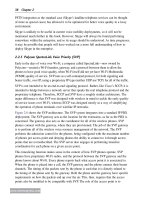
the other from the center frequency, and uses that drift to derive the original data. For car
radios, which are usually analog, that drift becomes the signal that is sent to the speakers.
There is a third type, phase modulation (PM or ΦM, as Φ is the custom mathematical
symbol for phase, measured in degrees from 0 to 360), which works by altering the phase
of the signal, or the offset of the carrier in time. Figure 5.16 shows phase modulation, and
how it compares to frequency modulation. Note how the phase modulated signal is offset—
in this example of simple of phase modulation, the modulated appears to be reflected
vertically, the result of its phase having been altered by 180 degrees—when the data signal
is non-zero, whereas the frequency modulated signal clearly has been sped up or slowed
down for non-zero data.
Because the phase of a signal is the offset from the carrier in degrees, and the amplitude is
just a distance the peak of the carrier is offset from the origin, an amplitude and phase
modulated signal can be represented using polar coordinates. In the descriptions here I will
try to avoid unnecessary mathematics, but the concept that the type of modulation applied
to a carrier can be represented by polar coordinates is powerful for those interested in
-1.0
-0.6
-0.2
0.2
0.6
1.0
0.0
0.2
0.4
0.6
0.8
1.0
-1.0
-0.6

-0.2
0.2
0.6
1.0
Carrier
Data Signal (between 0 and 1)
Final Modulated Signal = Data Signal × Carrier
Figure 5.14: Analog Amplitude Modulation
Introduction to Wi-Fi 151
www.newnespress.com
understanding just what radios do to the signal to be able to transmit the data. The polar
coordinate representation is one of the two common methods for representing complex
numbers, and the designs of radios are always though of as involving complex math. (A
complex number is type of number that can represents the square roots of negative numbers,
something not allowed in real numbers.) For those interested in the details, the appendix at
the end of this chapter explores the mathematics.
The term “baseband” refers to the signal converted into a function that, when multiplied by
the carrier, will produce the ultimate function. Therefore, the baseband signal can be
thought of as the encoded signal, but before any particular channel or center frequency has
been chosen. This means that the baseband signal is identical for every channel. Because
the baseband encoding is the most complicated part of the radio—it does the business of
giving the signal its flavor, if you will, the part of a radio that encodes or modulates the
signal is also called the baseband.
In digital systems, which 802.11 belongs to, phase modulation is known by the term phase
shift keying (PSK), representing that the phase is shifted abruptly because of the digital
-1.0
-0.6
-0.2
0.2
0.6

1.0
-1.0
-0.6
-0.2
0.2
0.6
1.0
-1.0
-0.6
-0.2
0.2
0.6
1.0
Carrier = A cos [2
p
f
c
t ]
Data Signal (between -1 and 1)
Final Modulated Signal = A cos [2
p
(f
c
+ Data) t ]
Figure 5.15: Analog Frequency Modulation
152 Chapter 5
www.newnespress.com
nature of the incoming signal, and the shift is “keyed” by the digital data. Understanding
these terms is not necessary to understanding Wi-Fi, but it can offer some insight into why
some radios do better in certain environments than others.

5.5.1.1 1Mbps
For 1Mbps, 802.11 uses what is called binary phase shift keying (BPSK). This simply
means that the phase is shifted forward by 180 degrees for a 1 bit in the data, and left
-1.0
-0.6
-0.2
0.2
0.6
1.0
-1.0
-0.6
-0.2
0.2
0.6
-1.0
-0.6
-0.2
0.2
0.6
Carrier = A cos [2p f
c
t ]
Data Signal (between -1 and 1)
NOTE: Because the phase modulation maps the incoming signal into the range of 180
degrees, plus or minus, the encoded signal can only differentate between a zero and
non-zero value. -1 and 1 become -180 degrees and 180 degrees, which are equal.
-1.0
-0.6
-0.2
0.2

0.6
Phase Modulated Signal = A cos [2p f
c t
+ Data]
Frequency Signal = A cos [2p (f
c
+ Data) t ]
Figure 5.16: Frequency versus Phase Modulation
Introduction to Wi-Fi 153
www.newnespress.com
The modulating signal, however, is not just the stream of bits that make up the frame.
Additional work goes in to prepare the incoming bitstream for transmission so that it will
better survive the sometimes nasty conditions of the RF channel. Each incoming data bit is
mapped to 11 transmission bits. These outgoing 11 bits are called, together, one symbol, and
each of the eleven bits is individually called a chip. The process of mapping bits to chips is
known spreading, the term deriving from the effect the mapping has of spreading out the
frequency range the signal takes on. (Or, one can think of the process as spreading the
information contained in the original data bit over the various chip bits of the symbol.) This
expanding of one data bit to 11 chip “bits” is done to protect the signal from various types
0°
180°
90°
-90°
A = 1
in-phase axis (I)
quadrature axis (Q)
xx
data = 0data = 1
Figure 5.17: Binary Phase Shift Keying
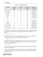
unmodified for a 0 bit in the data. Figure 5.17 shows what is called the constellation for this

representation. Don’t let it be intimidating: this is just the polar coordinate system
mentioned previously, with each X representing the modulation of the carrier represented by
each bit. Notice that the distance from the origin A is always 1: BPSK does not use
amplitude modulation at all.
154 Chapter 5
www.newnespress.com
of interference, and the mapping is very specific sequence known as a Barker sequence. The
sequence used happens to be
+1, −1, +1, +1, −1, +1, +1, +1, −1, −1, −1
where +1 represents the 1 bit and −1 represents the 0 bit. This sequence might seem to be
random, but it was chosen because it possesses an important real-world property. As the
signal encoded with this Barker sequence reflects off surfaces, it will be delayed a bit
relative to the original signal, and each delayed reflection that hits the receiver will appear
to be added together, causing the received signal to appear blurred out as the sequences
overlap. The important mathematical property of the Barker sequence is that the
autocorrelation, or the sum of the element-wise product of the sequence and any delayed
version of the sequence, will have a strong peak when no delay is present and will be close
to zero otherwise. This allows the receiver to use math to hunt out the main signal—the part
that comes directly from the transmitter and not off of reflected surfaces—and filter out the
echoes to get a cleaner signal. Furthermore, the increasing of the rate by a factor of 11
provides redundancy in time, which causes spreading in frequency to the final 20MHz
bandwidth. The advantage of spreading the signal over a wider range of frequencies is that
many interference sources are narrow-band and will then affect only a small part of the
encoded signal, rather than the entire signal, and the receiver may still be able to recover
the original data. See Figure 5.18.
-1
0
1
Eleven-chip Barker Sequence
+1

-1 -1
+1 +1 +1 +1 +1
-1 -1 -1
-2
11
Autocorrelation of Eleven-chip Barker Sequence
Figure 5.18: The 11-Chip Barker Code
Introduction to Wi-Fi 155
www.newnespress.com
Two more points: the data bits are differentially encoded, meaning that if two bits to send
are 11, the chip sequence is the Barker sequence, followed by the Barker sequence
multiplied by −1. The differential encoding is used to make it unnecessary for the receiver
to know whether 0 degrees is a 0 bit and 180 degrees is a 1 bit, or vice versa. Also, the data
bits go through a process known as scrambling, which ensures that data that is made of
predominantly one value—such as a string of zeros—has enough variation over the air to
prevent the signal from not changing enough and drifting to one side or the other of the
center frequency, something which makes the signal harder to transmit or receive. The
process is called scrambling because the bits are modified with a pseudorandom sequence—
there is no security aspect in this, however. The scrambled bits end up becoming the ones
that are then spread out into the 11-chip symbols.
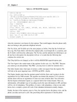
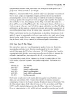
5.5.1.2 2Mbps
The 2Mbps data rate is very similar to the 1Mbps data rate. The main difference is that the
data bits are taken pairwise (after scrambling), and encoded so that two-bit pairs map to
11-chip symbols. This doubles the data rate: the two bits are packed in by encoding both
bits into one symbol, with the symbol taking the same time as a 1Mbps one. Looking at the
constellation (Figure 5.19), the four possible values of the two bits—00, 01, 10, and 11—
are equally spaced around the circle—at degrees 0, 90, 180, and 270 (-90). In this sense, the
two bits are packed in by splitting “space”, meaning room in the constellation, rather than
sending one after the other by splitting “time”.
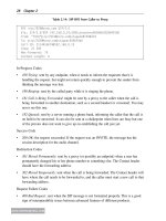
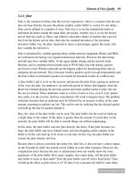
The downside to packing in two bits per symbol is that the distance between the

constellation points on the symbol has gone down. This is important, because noise
shows up at the receiver as an uncertainly about whether a given symbol belongs as one of
the—in this case, four Xs. If there are only two possible symbols, as with the 1Mbps rate,
then the receiver’s value would have had to have drifted very far to cause a mistake. With
four possible symbols, however, the received symbol need not drift as far to cause an error.
This is what was being referred to earlier when discussing how lower data rates are more
robust, whereas higher data rates require increased fidelity. The more noise, the worse the
higher data rates do, and the more mistakes they make. In 802.11, one mistake in choosing
the symbol causes the entire frame, good bits and bad, to be dropped as an error (Figure
5.20).
Therefore, the 2Mbps data rate requires both a higher absolute signal strength and a higher
SNR to be received, and thus will not carry with quite the same range as 1Mbps rates will.
5.5.1.3 5.5Mbps and 11Mbps
The 5.5Mbps data rate was the first one introduced in the 802.11b amendment itself.
Recognizing that 2Mbps was not fast, compared with the predominant 10Mbps wireline
speeds from 10BASE-T Ethernet, the IEEE introduced the 5.5Mbps and 11Mbps data rates.
156 Chapter 5
www.newnespress.com
To get to the faster data rate, IEEE decided not to continue splitting space by adding more
points to the constellation. Instead, they looked at the 11 chips, and decided to pack more
bits in by changing the data bits throughout the 11-chip sequence, thus splitting time.
Instead of assigning one or two bits for the entire 11-chip sequence, both 5.5Mbps and
11Mbps use an eight-chip sequence (still sent out at 11 megachips/second), and then map
either four or eight bits to each eight-chip symbol. These eight-chip symbols are QPSK
encoded, and the (complex) value of each of the eight chips is determined by four bit-pairs
that are input. The particular formula used to determine the eight chip values from the eight
input bits is designed to increase the reliability of the signal, and is a type of complementary
code keying (CCK).
The 11Mbps rate maps the eight data bits per symbol to the four bit-pairs directly. The
5.5Mbps data rate is produced by using only four data bits to get the eight-bit input to the

formula by using a specified mapping up front, adding greater redundancy.
Because of the greater redundancy, 5.5Mbps has a longer range and less SNR requirements
than 11Mbps.
0°180°
90°
-90°
A = 1
in-phase axis (I)
quadrature axis (Q)
x
x
x
x
data = 00
data = 01
data = 11
data = 10
Figure 5.19: Quadrature Phase Shift Keying
Introduction to Wi-Fi 157
www.newnespress.com
5.5.1.4 Short and Long Preambles
802.11b allows the transmitter to choose from either a short or long preamble for the 2, 5.5,
and 11Mbps data rates. The intent of allowing a short preamble, being almost exactly half
as short in time as the long preamble will be to free up some additional airtime, at the risk
of slightly decreasing the chances that there will be enough time for a radio to lock onto the
signal. In the early days of 802.11b-only networking, this statement may have been more
true. Now, however, most of the distinction is lost, and short preambles should always be
recommended, unless old legacy devices are in use. Most of the issues with short preambles
now are from those old devices not accepting short preambles.
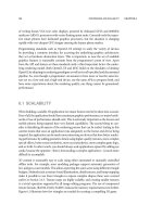
5.5.2 802.11a and 802.11g

802.11a and 802.11g expanded the data rates and network efficiency significantly, leading to
a top data rate of 54Mbps. 802.11a—for the 5GHz band—and 802.11g—for the 2.4GHz
band—are nearly identical except for the band in use and some additional rules. Their
introduction was a turning point in Wi-Fi, allowing the designers to use a newer, different
0°180°
90°
-90°
A = 1
in-phase axis (I)
error circles
This symbol will be
received correctly
This symbol is
ambiguous and will
probably be received
incorrectly
quadrature axis (Q)
x
x
x
x
*
*
data = 00
data = 01
data = 11
data = 10
Figure 5.20: Symbol Error
158 Chapter 5
www.newnespress.com

way of encoding signals than before that would greatly enhance the speed of the network,
as well as the robustness.
The challenge to 802.11 designers was to increase the data rates by packing more bits into
the channel, but without requiring the signal itself to fluctuate in time so fast that delay
effects prevented the radio from working in real environments. In fact, if there was a way to
make the signal even more robust to delay, that would be useful in getting Wi-Fi into more
environments with more reliability.
In the end, the designers settled on one scheme and gave them two letters. The two radios
use the same method to encode more data per symbol. This method works by dividing up
the channel from one 20MHz block to dozens of very small blocks, each of which becomes
its own miniature channel. This new technique is called orthogonal frequency division
multiplexing (OFDM). The frequency division part is rather straightforward: dividing the
20MHz channel into 48 of those small channels (subcarriers), separated 20MHz/64 =
5/16th MHz apart allows the 20MHz band to be used more efficiently. (It is important to
note that the subcarriers always belong to the same transmission, and are not to be thought
of as separate, usable channels.) The orthogonal aspect is that the subcarriers are encoded
and spaced so that the sidelobes, or parts of the subcarrier that would ordinarily interfere
with adjacent signals) do not interfere with adjacent subcarriers here. Why create more
carriers? 802.11b, at 1Mbps, has 1-microsecond symbols, which are relatively short in time.
To get to 11Mbps, 802.11b had to shrink the symbol to 73% the original duration and vary
the data within the symbol for each 90-nanosecond chip. Trying this for 54Mbps would
require either varying the data every 18 nanoseconds, or making major sacrifices on the
redundancy. Either way, the signal would not be able to travel through most environments
very well, and Wi-Fi would not be able to transmit at high speeds past a few feet. However,
by spreading the data out across 48 subcarriers, the data rate on each subcarrier is dropped
back to something similar to the 1Mbps 802.11b data rate—1.125Mbps. Bumping up the
modulation to six scrambled bits per symbol then allows the symbol to be held without
fluctuation for longer and reduces the bandwidth of the subcarrier to its final value, resulting
in a growth from 1 microsecond symbols to 4 microseconds. By packing in more bits per
Hz, the signal can become more resilient over time.

This advance was quite exciting for its time, and is still one of the two major underpinnings
for modern 802.11n radios.
Table 5.12 shows the data rates available to 802.11ag. There are now eight data rates unique
to 802.11ag.
The two additions to 802.11b for each subcarrier are the growth of the constellations and
the use of an error correction code built into the radio. The first part, the constellation
expansion, builds upon the concepts used to expand from 1Mbps to 2Mbps to pack more
Introduction to Wi-Fi 159
www.newnespress.com
bits in. The constellation points are no longer on a circle; rather, they are spaced evenly on
a square grid, with 64-QAM being more dense in both amplitudes and phases. Figure 5.21
shows the two constellations—this time, the labels for which bits go to which constellation
point are left off for clarity.
As you may notice, the use of four different modulation schemes—BPSK, QPSK, 16-QAM,
and 64-QAM—lead to four different numbers of coded bits per symbol, but there are eight,
not four, data rates. To allow for two data rates for the same modulation type, 802.11ag
introduces the error correction code. Error correction codes are methods of expanding digital
data into something with more bits than the original in such a way that some of those
expanded bits can be lost without causing a loss in the original data. In a pure sense, this is
the opposite goal from data compression, where redundant bits are removed, rather than
added. The extra bits are wasteful if there are no errors in the data, but if there are errors in
the data, the code will protect the data from loss. Redundancy in wireless, as we have seen, is
a good thing to have. We’ve seen spreading sequences already, and error correction codes can
be thought of as a way to spread the bits as well, but over time rather than over frequencies.
(Of course, frequency and time are two sides of the same coin.)
The simplest error correction codes are just to repeat bits of the data. A bit stream of
101101 can be doubled, to produce 101101101101. This stream protects against any one bit
being lost. Let’s say that the stream arrives at the receiver as 101x01101101, where x is the
lost bit. The receiver can clearly recover the lost bit, by looking at the copy that makes up
the second half of the transmission. Doubling protects the stream from up to 50% loss, if

the right 50% is lost, but can fail at two losses if the two bits lost are from the same source.
Because the ability to correct for errors depends not only on the number of bits lost, but the
positions of the lost bits, doubling makes for a very poor error-correction code in practice.
To protect against exactly one bit loss in the most efficient manner possible, just sum the
Table 5.12: The 802.11ag data rates
Speed Modulation Bits per Symbol per
Subcarrier
Coding Rate
6Mbps BPSK 1
1
2
9Mbps BPSK 1
3
4
12Mbps QPSK 2
1
2
18Mbps QPSK 2
3
4
24Mbps 16-QAM 4
1
2
36Mbps 16-QAM 4
3
4
48Mbps 64-QAM 6
2
3
56Mbps 64-QAM 6

3
4