Scalable voip mobility intedration and deployment- P21 pot

200 Chapter 5
www.newnespress.com
interference is not an issue. But when the channel leads to enough cross-stream interference,
MIMO can shut down.
5A.5 Why So Many Hs? Some Information Theory
For those readers curious as to why there are so many instances of the letter H in the
formulas, read on. HH
H
comes from attempting to maximize the amount of information that
the radio can get through the channel and into y by picking the best values of s. That
matters because H acts unevenly on each symbol. Some symbols may be relatively simple
and robust, and others may be more finicky and sensitive. The definition of information is
from information theory (and is purely mathematical in this context), and we are looking for
trying to maximize the amount of mutual information from what the transmitter sent (s) and
what the receiver got (y).
Intuitively, the measure of the maximum information something can carry is the amount of
different values the thing can take on. We are looking at y, and trying to see how much
information can be gleaned from it. The channel is something that removes information,
rather than, say, adding it. For MIMO, this removal can happen just by going out of range,
or by being in range but having a spatial stream that can’t get high SNR even though a
non-MIMO system would have that high SNR. The latter can only come from some form of
interference between the spatial streams.
To look at that, we need to look at the amount of stream-to-stream correlation that each
possible value of y can have. This correlation, across all possible values of y, is known as
the covariance of y, or cov(y), and can be represented by an N×N matrix. MIMO works
best when each of the antennas appears to be as independent as possible of the others. One
way of doing that would be for the covariance of one antenna’s signal signal y
i
with itself to
be as high as possible across all covalues of y, but for the covariance of a signal y
i

with a
signal y
j
from another antenna to be as close to zero as possible. The reason is that the
higher the covariance of an antenna’s signal with itself, the more variation from the mean
has been determined, and that’s what information looks like—variation from the mean.
When the other terms are zero, the cross-stream interference is also zero. A perfect MIMO
solution would be for every antenna on the receiver to connect directly with every antenna
on the transmitter by a cable. That would produce a covariance matrix with reasonable
numbers in the diagonal, for every antenna with itself, and zeros for every cross-correlation
between antennas.
The determinant of the covariance matrix measures the amount of interference across
antennas. The closer to 0 the determinant is, the more the interantenna interference degrades
the signal and reduces the amount of information available. The determinant is used here
because it can be thought of as defining a measure of just how independent the rows of a
Introduction to Wi-Fi 201
www.newnespress.com
matrix are. Let’s look at the following. The determinant of the identity matrix I, a matrix
where each row is orthogonal, and so the rows taken as vectors point as far away from the
others as possible, is 1. The determinant of a matrix where any two of the row or columns
are linearly dependant is 0. Other matrices with normalized rows fall in between those two,
up to a sign. Geometrically, the determinant measures the signed volume of the
parallelepiped contained within the matrix’s rows. The more spread out and orthogonal the
rows, the further the determinant gets from zero.
Because of equation (10), the covariance matrix for y is proportional to the covariance
matrix of s, with the effects of the channel applied to it through H, followed by a term
containing the noise. As an equation

cov covy H s H I
(

)
=
(
)
+E N
H
sT 0

(14)
where E
sT
is the average energy of the symbol per stream, and N
0
is the energy of the noise.
(Note that the noise’s covariance matrix is I, the identity matrix, because no two noise
values are alike, and thus two different noise values have a covariance of 0.)
Now, we begin to see where the HH
H
comes from: it is just a representation of how the
channel affects the symbol covariance matrix. As mentioned before, the amount of
information that is in the signal is the determinant of the covariance matrix cov(y). Dividing
out the noise value N
0
, the amount of mutual information in s and y becomes simply equal
to the number of bits (base-2 logarithm) of the determinant of cov(y), which, using (11),
gives us

capacity
sT
=

(
)
(
)
+
[ ]
lg det covE N
H
0
H s H I

(15)
Remember that we are looking at this from the point of view of how to make the best radio,
so we can pick whatever set of symbols we want. However, symbols are usually chosen so
that each symbol is as different as possible from the others, because the channel isn’t
known in advance and we are considering a general-purpose radio that should work well in
all environments. Therefore, no two symbols have strong covariance, and so, if you think of
cov(s) as being close to the identity matrix itself (zero off-diagonal, one on), we drop the
cov(s) = I and get

capacity E
sT
=
(
)
+
[ ]
lg det N
H
0

HH I

(16)
Going a bit deeper into linear algebra, we can extract the eigenvalues of the matrix HH
H
to
see what that matrix is doing. With a little math, we can see that the effect of HH
H
is to act,
for each spatial stream, like its own independent attenuator, providing attenuation equal to
the eigenvector for each spatial stream.
202 Chapter 5
www.newnespress.com

capacity sum of capacity for each spatial stream
E
sT
=
=
(
)
lg N
0
eeigenvector for i
(
)
+
[ ]
∑
1

(17)
Okay, a lot of math, with a few steps skipped. Let’s step back. The capacity for each of the
spatial stream is based on the signal-to-noise ratio for the symbol (E
sT
/N
0
) times how much
the combined effect HH
H
of the channel matrix has on that spatial stream. This itself is the
per-stream SNR, with the noise coming from the other streams. The more independent each
basis for HH
H
is, the more throughput you can get. And since HH
H
depends only on the
channel conditions and environments, we can see that capacity is directly dependant on how
independent the channel is. If the channel allows for three spatial streams, say, but one of
the spatial streams has such low SNR that it is useless, then the capacity is only that of two
streams and you should hope that the radio doesn’t try to use the third stream. And overall,
this dependence on the channel was what we sought out to understand.
203
CHAPTER 6
Voice Mobility over Wi-Fi
6.0 Introduction
In the previous chapter, you learned what Wi-Fi is made of. From here, we can look at
how the voice technologies from previous chapters are applied to produce voice mobility
over Wi-Fi.
The keys to voice mobility’s success over Wi-Fi are, rather simply, that voice be mobile,

high-quality, secure, and that the phones have a long talk and standby time. These are the
ingredients to taking Wi-Fi from a data network, good for checking email and other non-
real-time applications but not designed from the start to being a voice network, to being a
network that can readily handle the challenges of real-time communication.
It’s important to remember that this has always been the challenge of voice. The original
telegraph networks were excellent at carrying non-real-time telegrams. But to go from relay
stations and typists to a system that could dedicate lines for each real-time, uninterruptible
call, was a massive feat. Then, when digital telephony came on the scene, the solution was
to use strict, dedicated bandwidth allocation and rigorous and expensive time slicing
regimes. When voice moved to wired Ethernet, and hopped from circuit switching to packet
switching, the solution was to throw bandwidth at the problem or to dedicate parallel voice
networks, or both. Wi-Fi doesn’t have that option. There is not enough bandwidth, and
parallel networks—though still the foundation of many Wi-Fi network recommendations—
are increasingly becoming too expensive.
So, let’s look through what has been added to Wi-Fi over the years to make it a suitable
carrier for voice mobility.
6.0.1 Quality of Service with WMM—How Voice and Data Are Kept Separate
The first challenge is to address the unique nature of voice. Unlike data, which is usually
carried over protocols such as TCP that are good at making sure they take the available
bandwidth and nothing more, ensuring a continuous stream of data no matter what the
network conditions, voice is picky. One packet every 20 milliseconds. No more, no less.
The packets cannot be late, or the call becomes unusable as the callers are forced to wait for
©2010 Elsevier Inc. All rights reserved.
doi:10.1016/B978-1-85617-508-1.00001-3.
204 Chapter 6
www.newnespress.com
maddening periods before they hear the other side of their conversation come through. The
packets cannot arrive unpredictably, or else the buffers on the phones overrun and the call
becomes choppy and impossible to hear. And, of course, every lost packet is lost time and
lost sounds or words.

On Ethernet, as we have seen, the notion of 802.1p or Diffserv can be used to give
prioritization for voice traffic over data. When the routers or switches are congested, the
voice packets get to move through priority queues, ahead of the data traffic, thus ensuring
that their resources do not get starved, while still allowing the TCP-based data traffic to
continue, albeit at a possibly lesser rate.
A similar principle applies to Wi-Fi. The Wi-Fi Multimedia (WMM) specification lays out a
method for Wi-Fi networks to also prioritize traffic according to four common classes of
service, each known as an access category (AC):
• AC_VO:highest-priorityvoicetrafc
• AC_VI:medium-priorityvideotrafc
• AC_BE:standard-prioritydatatrafc,alsoknownas“besteffort”
• AC_BK:backgroundtrafc,thatmaybedisposedofwhenthenetworkiscongested
The underscore between the AC and the two-letter abbreviation is a part of the correct
designation,unfortunately.Youmaynotethattheterm“besteffort”appliestoonlyoneof
the four categories. Please keep in mind that all four access categories of Wi-Fi are really
best effort, but that the higher-priority categories get a better effort than the lower ones.
We’ll discuss the consequences of this shortly.
The access category for each packet is specified using either 802.1p tagging, when available
and supported by the access point, or by the use of Diffserv Code Points (DSCP), which are
carried in the IP header of each packet. DSCP is the more common protocol, because the
per-packet tags do not require any complexity on the wired network, and are able to survive
multiple router hops with ease. In other words, DSCP tags survive crossing through every
network equipment that is not aware of DSCP tags, whereas 802.1p requires 802.1p-aware
linksthroughoutthenetwork,allcarriedover802.1QVLANlinks.
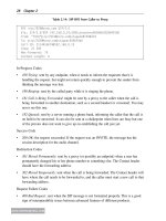
There are eight DSCP tags, which map to the four access categories. The application that
generates the traffic is responsible for filling in the DSCP tag. The standard mapping is
given in Table 6.1.
Thereareafewthingstonotehere.Firstisthattheeight“priorities”—again,thecorrect
term, unfortunately—map to only four truly different classes. There is no difference in
quality of service between Priority 7 and Priority 6 traffic. This was done to simplify the

design of Wi-Fi, in which it was felt that four classes are enough. The next thing to note is
Voice Mobility over Wi-Fi 205
www.newnespress.com
that the many packet capture analyzers will still show the one-byte DSCP field in the IP
header as the older TOS interpretation. Therefore, the values in the TOS column will be
meaningless in the old TOS interpretation, but you can look for those specific values and
map them back to the necessary ACs. Even the DSCP field itself has a lot of possibilities;
nonetheless, you should count on only the previous eight values as having any meaning for
Wi-Fi, unless the documentation in your equipment explicitly states otherwise. Finally, note
that the default value of 0 maps to best effort data, as does the Priority 3 (DSCP 0x18)
value. This strange inversion, where background traffic, with an actual lower over-the-air
priority, has a higher Priority code value than the default best effort traffic, can cause some
confusion when used; thankfully, most applications do not use Priority 3 and its use is not
recommended here as well.
A word of warning about DSCP and WMM. The DSCP codes listed in Table 6.1 are neither
Expedited Forwarding or Assured Forwarding codes, but rather use the backward-
compatibility requirement in DSCP for TOS precedence. TOS precedence, as mentioned in
Chapter 4, uses the top three bits of the DSCP to represent the priorities in Table 6.1, and
assign other meanings to the lower bits. If a device is using the one-byte DSCP field as a
TOS field, WMM devices may or may not ignore the lower bits, and so can sometimes give
no quality-of-service for tagged packets. Further complicating the situation are endpoints
that generate Expedited Forwarding DSCP tags (with code value of 46). Expedited
Forwarding is the tag that devices use when they want to provide higher quality of service
in general, and thus will usually mark all quality-of-service packets as EF, and all best effort
packets with DSCP of 0. The EF code of 46 maps, however, to the Priority value of 5—a
video, not voice, category. Thus, WMM devices may map all packets tagged with Expedited
Forwarding as video. A wireless protocol analyzer shows exactly what the mapping is for
by looking at the value of the TID/Access Category field in the WMM header. The WMM
header is shown in Table 5.5.
This mapping can be configured on some devices. However, changing these values from the

defaults can cause problems with the more advanced pieces of WMM, such as WMM
Table 6.1: DSCP tags and AC mappings
DSCP TOS Field Value Priority Traffic Type AC
0x38 (56) 0xE0 (224) 7 Voice AC_VO
0x30 (48) 0xC0 (192) 6 Voice AC_VO
0x28 (40) 0xA0 (160) 5 Video AC_VI
0x20 (32) 0x80 (128) 4 Video AC_VI
0x18 (24) 0x60 (96) 3 Best Effort AC_BE
0x10 (16) 0x40 (64) 2 Background AC_BK
0x08 (8) 0x20 (32) 1 Background AC_BK
0x00 (0) 0x00 (0) 0 Best Effort AC_BE
206 Chapter 6
www.newnespress.com
Power Save and WMM Admission Control, so it is not recommended to make those
changes. (The specific problem that would happen is that the mobile device is required to
know what priority the other side of the call will be sending to it, and if the network
changes it in between, then the protocols will get confused and not put the downstream
traffic into the right buckets.)
Once the Wi-Fi device—the access point or the client—has the packet and knows its tag, it
will assign the packet into one of four priority queues, based on the access categories.
However, these queues are not like their wired Ethernet brethren. That is because it is not
enough that voice be prioritized over data within the device; voice must also be prioritized
over the air.
To achieve this, WMM changes the backoff procedure mentioned in Section 5.4.8. Instead
of each device waiting a random time less than some interval fixed in the standard, each
device’s access category gets to contend for the air individually. Furthermore, to get the
over-the-air prioritization, higher quality-of-service access categories, such as voice, get
more aggressive access parameters.
Each access category get four parameters that each determine how much priority the traffic
in that category gets over the air, compared to the other categories. The first parameter is a

unique per-packet minimum wait time called the Arbitration Interframe Spacing (AIFS).
This parameter is the minimum amount of time that a packet in this category must wait
before it can even start to back off. The longer the AIFS, the more a packet must wait, and
the more it is likely that a higher-priority packet will have finished its backoff cycle and
started transmitting. The key about the AIFS is that it is counted after every time the
medium is busy. That means that a packet with a very high AIFS could wait a very long
time, because the amount of time spent waiting for an AIFS does not count if the medium
becomes busy in the meantime. The AIFS is measured in units of the number of slots, and
thus is also called the AIFSn (AIFS number).
The second value is the minimum backoff CW, called the CWmin. This sets the minimum
number of slots that the backoff counter for this particular AC must start with. As with
pre-WMM Wi-Fi, the CW is not the exact number of slots that the client must wait, but the
maximum number of slots that the packet must wait: the packet waits a random number of
slots less than this value. The difference is that there is a different CWmin for each access
category. The CWmin is still measured in slots, but communicated to the client from the
access point as the exponent of the power of two that it must equal. This exponent is called
the ECWmin. Thus, if the ECWmin for video is 3, then the AC must pick a random number
between 0 and 2
3
− 1 = 7 slots. The CWmin is just as powerful as the AIFS in
distinguishing traffic, by making access more aggressive by capping the number of slots the
AC must wait to send its traffic.
The third parameter is similar to the minimum backoff CW, and is called the CWmax, or
the maximum backoff CW. If you recall, the CW is required to double every time the
Voice Mobility over Wi-Fi 207
www.newnespress.com
sender fails to get an acknowledgement for a frame. However, that doubling is capped by
the CWmax. This parameter is far mess powerful for controlling how much priority one AC
gets over the other. As with the CWmin, there is a different CWmax for each AC.
The last parameter is how many microseconds the AC can burst out packets, before it has to

yield the channel. This is known as the Transmit Opportunity Limit
(TXOPLimit),andis
measured in units of 32 microseconds (although user interfaces may show the microsecond
equivalent). This notion of TXOPs is new with WMM, and is designed to allow for this
bursting. For voice, bursting is usually not necessary or useful, because voice packets come
on regular, well-spaced intervals, and rarely come back-to-back in properly functioning
networks.
The access point has the ability to set these four AC parameters for every device in the
network, by broadcasting the parameters to all of the clients. Every client, thus, has to share
the same parameters. The access point may also have a different set for itself. Some access
points set these values by themselves to optimize network access; others expose them to the
user, who can manually override the defaults. The method that WMM uses to set these
values to the clients is through the WMM Parameter Set information element, a structure
that is present in every beacon, and can be seen clearly with a wireless packet capture
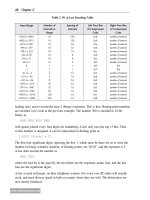
system. Table 6.2 has the defaults for the WMM parameters.
Table 6.2: Common default values for the WMM parameters for 802.11
AC Client Access Point CWmin TXOP limit
AIFS CWmax AIFS CWmax 802.11b 802.11agn
Background
(BK)
7
2
10
− 1 =
1023
7
2
10
− 1 =
1023

2
4
− 1 =
15
0µs 0µs
Best Effort
(BE)
3
2
10
− 1 =
1023
3
2
6
− 1 = 63 2
4
− 1 =
15
0µs 0µs
Video (VI) 2
2
4
− 1 = 15
1
2
4
− 1 = 15 2
3
− 1 = 7 6016µs 3008µs

Voice (VO) 2
2
3
− 1 = 7
1
2
3
− 1 = 7 2
2
− 1 = 3 3264µs 1504µs
6.0.1.1 How WMM Works
The numbers in Table 6.2 seem mysterious, and it is not easy to directly see what the
consequences are by WMM creating multiple queues that act to access the air
independently. But it is important to understand what makes WMM works, to understand
how WMM—and thus, voice—scales in the network.
LookingatthecommonWMMparameters,wecanseethatthemainwaythatWMM
provides priority for voice is by letting voice use a faster backoff process than data. The
shorter AIFS helps, by giving voice a small chance of transmitting before data even gets a
208 Chapter 6
www.newnespress.com
chance, but the main mechanism is by allowing voice transmit, on average, with a quarter
of the waiting time that best effort data has.
This mechanism works quite well when there is a small amount of voice traffic on a
network with a potentially large amount of data. As long as voice traffic is scarce, any given
voice packet is much more likely to get on the air as soon as it is ready, causing data to
build up as a lower priority. This is one of the consequences of having different queues for
traffic. As an analogy, picture the security lines at airports. Busy airports usually have two
separate lines, one line for the average traveler, and another line for first-class passengers
andthosewhoyenoughtogain“elite”statusontheairlines.Whenthelineforthe
averagetraveler—the“besteffort”line—isfullofpeople,ashortlineforrstclass

passengers gives those passengers a real advantage. In other words, we can think of best
effort and voice as mostly independent. The problem, then, is if there are too many first-
classpassengers.ForWMM,theproblemhappenswhenthereis“toomuch”voicetrafc.
UnlikewiththechildrenofLakeWobegone,noteveryonecanbeaboveaverage.
Let’slookatthismoremethodically.FromSection5.4.8,wesawthatthebackoffvalueis
the primary mechanism that Wi-Fi is affected by density. As the number of clients increases,
the chance of collision increases. Unfortunately, WMM provides for quality of service by
reducing the number of slots of the backoff, thus making the network more sensitive to
density. Again, if voice is rare, then its own density is low, and so a voice packet is not
likely to collide with other voice packets, and the aggressive backoff settings for voice,
compared to data, allow for voice to get on the network with higher probability. However,
when the density of voice goes up, the aggressive voice backoff settings cause each voice
packet to fight with the other voice packets, leading to more collisions and higher loss.
One solution for this problem is to limit the number of voice calls in a cell, thus ensuring
that the density of voice never gets that high. This is called admission control, and is
described in Section 6.1.1. Another and an independent solution is for the system to provide
a more deterministic quality of service, by intelligently setting the WMM parameters away
from the defaults. This exact purpose is envisioned by the standard, but most equipment
today expects the user to hand-tune these values, something which is not easy. Some
guidelines are provided in Section 6.4.1.2.
6.0.2 Battery Life and Power Saving
On top of quality of service, voice mobility devices are usually battery-operated, and
finding ways of saving that battery life is paramount to a good user experience.
The main idea behind Wi-Fi power saving is that the mobile device’s receive radio doesn’t
really need to always be turned on. Why the receive radio? Although the transmit side of
the radio takes more power, because it has to actually send the signal, it is used only when
Voice Mobility over Wi-Fi 209
www.newnespress.com
the device has something to send. The receive side, on the other hand, would always have
to be on, slowly burning power in the background, listening to every one of the thousands

of packets per second going over the air. If, at the end of receiving the packet, it turns out
that the packet was for the mobile device, then good. But, if the packet was for someone
else, the power was wasted. Adding up the power taken for receiving other device’s packets
to the power needed just to check whether a signal is on the air leads to a power draw that
is too high for most battery-operated devices.
When the mobile device is not in a call—when it is in standby mode—the only real
functions the phone should be doing are maintaining its connection to the network and
listening for an incoming call. When the device is in a call, it still should be sleeping during
the times between the voice packets. Thus, Wi-Fi has two modes of power saving, as
described in the following sections.
6.0.2.1 Legacy Power Save
The first mode, known as legacy power saving because it was the original power saving
technique for Wi-Fi, is used for saving battery during standby operation.
This power save mode is not designed for quality-of-service applications, but rather for data
applications. The way it works is that the mobile device tells the access point when it is
going to sleep. After that time, the access point buffers up frames directed to the mobile
device, and sets a bit in the beacon to advertise when one or more frames are buffered. The
mobile device is expected to wake every so many beacons and look for its bit set in the
beacon. When the bit is set, the client then uses one of two mechanisms to get the access
point to send the buffered frames.
This sort of system can be thought of as a paging mechanism, as the client is told when the
access point has data for it—such as notification of an incoming call. Figure 6.1 shows the
basics of the protocol.
The most important part of the protocol is the paging itself. Each client is assigned an
association ID (AID) when it associates. The value is given out by the access point, in a
field in the Association Response that it sent out when the client connected to it. The AID
is a number from 1 to 2007 (an extremely high number for an access point) that is used by
the client to figure out what bit to look at in the beacon. Each beacon carries a Traffic
Indication Map (TIM), which is an abbreviated bit field. Each client who has a frame
buffered for it has its bit set in the TIM, based on the AID. For example, if a client with

AID of 10 has one or more frames buffered for it, the tenth bit (counting from zero) of the
TIM would be set.
Because beacons are set periodically, using specific timing that ensures that it never goes
out before its time, each client can plan on the earliest it needs to wake up to hear the