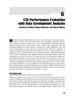
Commodity Trading Advisors: Risk, Performance Analysis, and Selection Chapter 9 ppt

CHAPTER
9
CHAPTER 9
Measuring the Long Volatility
Strategies of Managed Futures
Mark Anson and Ho Ho
C
ertain hedge fund strategies create investment positions that resemble a
long put option. Specifically, managed futures or commodity trading
advisors have significant exposure to volatility events. This exposure is pos-
itively related to volatility much like a long option position. We identify and
measure this long volatility exposure, which may not always be transparent
from the trading positions of a commodity trading advisor. We also examine
ways to apply these long volatility strategies to improve risk management.
INTRODUCTION
The managed futures industry has come full circle in its application over the
last 15 years. In the early 1990s, global macro funds were the predominant
form of the hedge fund industry. These funds were primarily managed
futures funds run by commodity trading advisors (CTAs). As the 1990s pro-
gressed, other types of hedge fund strategies came to the forefront, such as
relative value arbitrage, event driven, merger arbitrage, and equity long/short.
As these strategies grew, managed futures became a smaller part of the
hedge fund industry.
Now, however, managed futures have achieved a renewed interest
because of their risk reducing properties relative to other hedge fund strate-
gies. Specifically, most CTA strategies employ some form of trend-following
strategy. These trend-following strategies pursue both up- and down-market
movements in futures markets. These strategies also may be called momen-
tum strategies because they follow the momentum of the market and then
liquidate their positions (or reverse them) when they detect that the momen-
tum is changing or about to change.

183
c09_gregoriou.qxd 7/27/04 11:15 AM Page 183
Whether we call managed futures trend-following or momentum stra-
tegies, they have one important characteristic: They capitalize on the volatility
in the futures market. Trend-following strategies tend to be “long-volatility”
strategies; that is, they profit during volatile markets. Long-volatility strate-
gies can be useful risk management tools for other active trading strategies
that tend to be short volatility.
We begin with a brief overview of the managed futures industry. We
then measure the long-volatility exposure captured these strategies. Next
we apply Monte Carlo simulation to estimate the value at risk for long-
volatility strategies. Last, we demonstrate some practical risk management
strategies that may be employed with managed futures.
BRIEF REVIEW OF THE MANAGED FUTURES INDUSTRY
Managed futures is often referred to as an absolute return strategy because
their return expectations are not driven by broad market indices, such as
the Standard & Poor’s (S&P) 500, but instead by the specialized trading
strategy of the commodity trading advisor. More specifically, their return
expectations are an absolute level of return sufficient to compensate them
for the risk associated with trading in the futures markets. This absolute
level is established independently of the return on the stock market.
The managed futures industry is another skill-based style of investing
similar to hedge fund managers. In fact, managed futures is considered a
subset of the hedge fund world. Commodity trading advisors use their spe-
cial knowledge and insight in buying and selling futures and forward con-
tracts to extract a positive return. This skill and insight can be applied
regardless of whether the stock or bond markets are rising or falling, pro-
viding the absolute return benefits described above.
Commodity trading advisors have one goal in mind: to capitalize on
price trends in futures markets. Typically, CTAs look at various moving aver-

ages of commodity prices and attempt to determine whether the price will
continue to trend up or down, and then trade accordingly. Some CTAs also
use volatility models such GARCH (generalized auto-regressive conditional
heteroskedasticity) to forecast both price trends and volatility changes.
Prior empirical studies have indicated that managed futures, or com-
modity trading advisors, have investment strategies that tend to be long
volatility. Fung and Hsieh (1997a) found that trend-following styles have a
return profile similar to a long option straddle position—a long volatility
position. Fung and Hsieh (1997b) documented that commodity trading
advisors apply predominantly trend-following strategies.
184 RISK AND MANAGED FUTURES INVESTING
c09_gregoriou.qxd 7/27/04 11:15 AM Page 184
In our research we use three Barclay Commodity Trading Advisor
indices to capture the trading dynamics of the CTA market: Commodity
Trading Index, Diversified Commodity Trading Advisor Index, and System-
atic Trading Index. These indices are an equally weighted average of a group
of CTAs who identify themselves as belonging to one of the three strategies.
There are alternative ways to gain exposure to the futures markets
without the use of a CTA. One way is a passive managed futures index,
such as the Mount Lucas Management Index (MLMI).
The MLMI applies a mechanical trading rule for following the price
trends in several futures markets. It uses a 12-month look-back window to
calculate the moving average unit asset value for each futures market in
which it invests. Once a month, on the day prior to the last trading day of
the month, the algorithm examines the current unit asset value in each
futures market compared to the average value for the prior 12-month
period. If the current unit asset value is above the 12-month average, the
MLMI purchases the futures contract. If the current unit asset value is
below the 12-month moving average, the MLMI takes a short position in
the futures contract.

The MLMI invests in and is equally weighted across 25 futures con-
tracts in seven major commodity futures categories: grains, livestock,
energy, metals, food and fiber, financials, and currencies. The purpose of its
construction is to capture the pricing trend of each commodity futures con-
tract without regard to its production value or trading volume in the market.
Our next step is to document the long volatility strategy of the man-
aged futures industry.
DEMONSTRATION OF A LONG VOLATILITY STRATEGY
In this section we use the direction of the stock market to demonstrate the
asymmetric payout associated with managed futures. That is, we expect
that large downward movements in the stock market will result in large
gains from managed futures. Conversely, we expect that large positive
movements in the stock market will result in a constant return to managed
futures. This type of return pattern is consistent with a long put option
exposure. Therefore, this section plots the direction of the stock market ver-
sus the returns earned by managed futures. In the “Mimicking Portfolios”
section we specifically incorporate a measure of volatility to determine its
impact on these hedge fund strategies.
We start by producing a scatter plot of the excess return to the Barclay
Commodity Trading Index returns versus the excess returns to the Standard
Measuring the Long Volatility Strategies of Managed Futures 185
c09_gregoriou.qxd 7/27/04 11:15 AM Page 185
& Poor’s (S&P) 100.
1
We use the S&P 100 because this is the underlying
index for which the VIX volatility index is calculated. We use the VIX index
in the next section. Figure 9.1 presents this scatter plot.
On the scatter plot in Figure 9.1, we overlay a regression line of the
excess return to the Barclay Commodity Trading Index on the excess
return to the S&P 100. Note that the fitted regression line is “kinked.” The

kink indicates that there are really two different relationships between the
excess returns to the stock market and the excess returns to managed
futures.
To the right of the kink, the relationship between the returns earned by
the CTAs and the stock market appears orthogonal. That is, there is no
apparent relationship between the returns to CTAs who pursue a diversified
trading program and the returns to the stock market, when the returns to
the stock market are positive.
When the stock market earns positive returns, the Commodity Trading
Index earns a consistent return regardless of how positive the stock market
186 RISK AND MANAGED FUTURES INVESTING
–8.00%
–6.00%
–4.00%
–2.00%
0.00%
2.00%
4.00%
6.00%
8.00%
10.00%
12.00%
–20.00% –15.00% –10.00% –5.00% 0.00% 5.00% 10.00% 15.00%
S&P 100 Excess Returns
CTA Excess Returns
CTA
Regression Line
FIGURE 9.1 Barclay Commodity Trading Index
1
Excess return is simply the total return minus the current risk-free rate.

c09_gregoriou.qxd 7/27/04 11:15 AM Page 186
performs. This part of the graphed line is flat, indicating a constant, con-
sistent return to managed futures when the stock market earns positive
returns. In this part of the graph, the excess return provided by the Com-
modity Trading Index is almost zero. That is, after taking into account the
opportunity cost of capital (investing cash in treasury bills), the return to
this style of managed futures is effectively zero, when there is no volatility
event. This result highlights a point about the managed futures industry: It
is a zero-sum game, similar to Newton’s law of physics: For every action,
there is an equal and opposite reaction.
However, to the left side of the kink, there is a distinct linear relation-
ship between the returns to managed futures and the S&P 100. Declines in
the stock market driven by volatility events result in large, positive returns
for the Barclay Commodity Trading Index. In fact, the fitted regression line
in Figure 9.1 mirrors the payoff function for a long put option.
Figures 9.2 through 9.4 demonstrate a similar “kinked” relationship
for the Barclay Diversified Trading Index, Systematic Trading Index, and
the MLMI. Each figure demonstrates a long put optionlike exposure. In the
next section, we examine how this kinked relationship can be quantified.
Measuring the Long Volatility Strategies of Managed Futures 187
–10.00%
–5.00%
0.00%
5.00%
10.00%
15.00%
–20.00% –15.00% –10.00% –5.00% 0.00% 5.00% 10.00% 15.00%
S&P 100 Excess Returns
Diversified Excess Returns
Diversified Trading

Re
g
ression Line
FIGURE 9.2 Barclay Diversified Trading Index
c09_gregoriou.qxd 7/27/04 11:15 AM Page 187
188 RISK AND MANAGED FUTURES INVESTING
–0.100
–0.050
0.000
0.050
0.100
0.150
0.200
–0.175 –0.150 –0.125 –0.100 –0.075 –0.050 –0.025 0.000 0.025 0.050 0.075 0.100 0.125
S&P 100 Excess Returns
Systematic Excess Returns
Systematic Trading
Re
g
ression Line
FIGURE 9.3 Barclay Systematic Trading Index
–0.080
–0.060
–0.040
–0.020
0.000
0.020
0.040
0.060
–0.175 –0.150 –0.125 –0.100 –0.075 –0.050 –0.025 0.000 0.025 0.050 0.075 0.100 0.125

S&P 100 Excess Returns
MLMI Excess Returns
MLM Index
Regression Line
FIGURE 9.4 MLM Index
c09_gregoriou.qxd 7/27/04 11:15 AM Page 188
FITTING THE REGRESSION LINE
The previous discussion provides a general framework in which to describe
empirically the long volatility exposure embedded within CTA trend-
following strategies. To fit the kinked regression demonstrated in Figures
9.1 through 9.4, we use a piecewise linear capital asset pricing model
(CAPM)–type model. The model can be described as:
R
tf
− R
f
= (1 − D)[a
low
+ b
low
(R
OEX
− R
f
)] +
D[a
high
+ b
high
(R

OEX
− R
f
)]
(9.1)
where
R
tf
= return to the trend-following strategy
R
f
= risk-free rate
R
OEX
= return to the S&P 100
a
low
, b
low
= regression coefficients to the left-hand side of the kink
a
high
, b
high
= regression coefficients to the right-hand side of the kink
D = 1 if R
OEX
− R
f
> the threshold

D = 0 if R
OEX
− R
f
< or equal to the threshold.
In essence we plot two regression lines that have different alpha and
beta coefficients depending on which side of the kink the market returns
fall. The trick is to maintain continuity at the kink in the fitted regression
line. To insure this, we impose this following condition:
a
low
+ b
low
(Threshold) = a
high
+ b
high
(Threshold) (9.2)
Our regression equation then becomes:
R
tf
− R
f
= (1 − D)[a
low
+ b
low
(R
OEX
− R

f
)] +
D[a
low
+ (b
low
− b
high
)(Threshold) + b
high
(R
OEX
− R
f
)]
(9.3)
We express our regression equation in this fashion to demonstrate how the
threshold value is explicitly incorporated into the solution. Table 9.1 pres-
ents the results for our fitted regression lines.
For the Barclay Commodity Trading Index, the threshold value (the
kink) is −5.2 percent.
2
Several observations can be made from the regresion
Measuring the Long Volatility Strategies of Managed Futures 189
2
We found the threshold value through a recursive method that minimizes the
residual sum of squares in equation 9.3.
c09_gregoriou.qxd 7/27/04 11:15 AM Page 189
TABLE 9.1 Two-Step Regression Coefficients
Commodity Trading Diversified Trading Systematic Trading MLM Index

Coefficient t-statistic Coefficient t-statistic Coefficient t-statistic Coefficient t-statistic
Threshold −0.0526 −0.0868 −0.0485 −0.0926
Alpha_low −0.0158 −1.2699 −0.0793 −1.7150 −0.0175 −1.2127 −0.0437 −1.7743
Beta_low −0.3962 −2.1083 −1.1018 −2.1911 −0.4923 −2.1703 −0.5893 −2.3223
Alpha_high 0.0014 0.0043 0.0029 0.0022
Beta_high −0.0676 −1.1759 −0.1384 −2.0820 −0.0717 −0.9365 −0.0929 −3.2138
S.E. 0.0264 0.0353 0.0343 0.0155
Regression
R square 0.0555 0.0745 0.0520 0.1203
Adj R square 0.0437 0.0629 0.0402 0.1094
190
c09_gregoriou.qxd 7/27/04 11:15 AM Page 190
coefficients. First, the value of b
low
is negative and significant at the 5 per-
cent level, with a t-statistic of −2.11. This demonstrates that when the
returns to the S&P 100 are negative, the commodity trading strategies earn
positive excess returns. In particular, the value of b
low
is −0.396, indicating
that CTAs earn, on average, about a 0.4 percent excess return for every 1
percent decline in the S&P 100 below the threshold value.
This is similar to a put option being exercised by the CTA manager
when the returns to the stock market are negative, but created synthetically
as a consequence of the trend-following strategy. As long as stock market
returns remain positive, CTAs earn a constant return equal to a cash (treas-
ury bill) rate. However, when the stock market suffers a negative volatility
event that drives market returns into negative territory, the synthetic put
option is exercised, leading to large positive returns.
The coefficient for b

high
is close to zero (−0.067). It is neither econom-
ically nor statistically significant.
3
Trend-following CTAs do not earn excess
returns when the returns to the stock market are positive. When the returns
to the S&P 100 are positive, there is no need to exercise the put option. In
addition, a
high
is also close to zero, indicating a lack of excess returns over
this part of the graph. Managed futures earn a treasury bill rate of return
when the returns to the stock market are positive. The lack of any excess
return over this part of the graph can be considered the payment for the put
option premium. That is, trend-following CTAs forgo excess returns when
the returns to the stock market are positive in return for a long put option
exposure to be exercised when the returns to the stock market are negative.
Similar results are presented in Table 9.1 for diversified trading man-
aged futures, systematic trading, and the passive MLMI index. In each case,
b
low
is economically and statistically significant. In addition, b
low
always
has a negative sign, indicating positive returns to managed futures when the
stock market earns negative returns. Also, a
high
is close to zero for each cat-
egory of managed futures. Once again, this indicates that managed futures
do not generate any excess returns when the returns to the stock market are
positive. All that is received is a cash return equal to treasury bills.

b
high
is statistically significant in two categories: diversified trading and
the MLMI. The sign of the b
high
is negative, indicating a downward slop-
ing curve. However, the coefficient is small and lacks economic significance.
Still, this indicates that managed futures can be countercyclical when the
stock market has positive returns.
Measuring the Long Volatility Strategies of Managed Futures 191
3
There is no t-statistic for a
high
because this coefficient is a linear combination of
the other regression coefficients (see equation 9.2).
c09_gregoriou.qxd 7/27/04 11:15 AM Page 191
MIMICKING PORTFOLIO
Here we specifically incorporate the long volatility exposure trend-following
strategies to build mimicking portfolios of the strategies. The idea is that if
we can build portfolios of securities that mimic the returns to CTAs, we can
then simulate how trend-following strategies should perform under various
market conditions.
We use three components to build the mimicking portfolios: long OEX
(options ticker symbol for S&P 100) put options, long the S&P 100 index,
and long the one-month risk-free treasury security. The long OEX put option
is used to capture the synthetic long put option exposure. The long S&P 100
index is used to capture any residual market risk that exists when the mar-
ket performs positively. Last, we use the risk-free rate to measure the option
premium that must be paid by CTAs to the right-hand side of the threshold
value (when the stock market performs positively). We use the coefficient

estimates from equation 9.3 to construct the mimicking portfolio.
Long OEX Put Option
Strike = OEX index × (1 + Threshold + risk-free rate)
Volatility = VIX index
The number of options bought = (b
low
− b
high
)
Short the S&P 100
4
The number of S&P 100 to buy is = b
high
Long Risk-Free Security
The number of risk-free securities to buy = 1 − b
low
Figures 9.5 through 9.8 present the results from our mimicking portfo-
lios. Similar to Figure 9.1, Figure 9.5 contains the scatter plot of the excess
returns earned by the Barclay Commodity Trading Index plotted against the
excess returns of the S&P 100. In addition, it contains the return of our
mimicking portfolio.
192 RISK AND MANAGED FUTURES INVESTING
4
Since the beta (high) is negative, a short amount of a negative number is equal to
a long position in the stock market.
c09_gregoriou.qxd 7/27/04 11:15 AM Page 192
Our mimicking portfolio performs relatively well and has the same
characteristics of the fitted regression line in Figure 9.1. First, the mimick-
ing portfolio has a distinct “kink” in its shape. Additionally, the slope of the
mimicking portfolio is flat to the right-hand side of the kink and has a neg-

ative slope to the left-hand side of the kink. In sum, our mimicking portfo-
lio captures the upside of a long put option exposure.
Figures 9.6 to 9.8 provide similar information for the other trend-
following strategies. We can see in each case that to the right of the kink,
there is a negative slope to our mimicking portfolio, just as there was for
the fitted regression lines. Each mimicking portfolio demonstrates a long
put option exposure.
In summary, we are able to build mimicking portfolios using traditional
securities that mimic the return patterns of trend-following CTA strategies.
Specifically, these mimicking portfolios capture both the long volatility
exposure of a long put option as well as the premium payment when all per-
forms well. Our next step is to provide some Value at Risk analysis.
Measuring the Long Volatility Strategies of Managed Futures 193
–8.00%
–6.00%
–4.00%
–2.00%
0.00%
2.00%
4.00%
6.00%
8.00%
10.00%
12.00%
–20.00% –15.00% –10.00% –5.00% 0.00% 5.00% 10.00% 15.00%
S&P 100 Excess Returns
CTA Excess Returns
CTA
Mimickin
g

Portfolio
FIGURE 9.5 Mimicking Portfolio Returns for the Barclay Commodity Trading
Index
c09_gregoriou.qxd 7/27/04 11:15 AM Page 193
194 RISK AND MANAGED FUTURES INVESTING
–10.00%
–5.00%
0.00%
5.00%
10.00%
15.00%
–20.00% –15.00% –10.00% –5.00% 0.00% 5.00% 10.00% 15.00%
S&P 100 Excess Returns
Diversified Excess Returns
Diversified Trading
Mimickin
g
Portfolio
FIGURE 9.6 Mimicking Portfolio Returns for the Barclay Diversified Trading Index
–0.100
–0.050
0.000
0.050
0.100
0.150
0.200
–0.175 –0.150 –0.125 –0.100 –0.075 –0.050 –0.025 0.000 0.025 0.050 0.075 0.100 0.125
S&P 100 Excess Returns
Systematic Trading
Mimicking Portfolio

Systematic Excess Returns
FIGURE 9.7 Mimicking Portfolio Returns for the Barclay Systematic Trading Index
c09_gregoriou.qxd 7/27/04 11:15 AM Page 194
VALUE AT RISK FOR MANAGED FUTURES
The main reason for building mimicking portfolios is to simulate the
returns to trend-following strategies for developing risk estimates. Specifi-
cally, we can run Monte Carlo simulations with our mimicking portfolios
and estimate value at risk (VaR). Armed with these data, we can estimate
the probability of the risk of loss associated with long volatility strategies.
This is important to help us understand the off-balance sheet risks associ-
ated with trend-following strategies.
In addition, we can use Monte Carlo simulations to graph the fre-
quency distribution of returns. Doing so allows us to demonstrate pictori-
ally the return patterns associated with long volatility strategies. A review
of these return patterns can provide some sense of the downside risk of loss.
Using the mimicking portfolios we run 10,000 simulations for the managed
futures strategies. Table 9.2 presents the results.
For example, the one-month VaR for the Barclay Commodity Trading
Index is −0.93 percent at a 1 percent confidence level and −0.69 percent at
a 5 percent confidence level. This means that we can state with a 99 per-
Measuring the Long Volatility Strategies of Managed Futures 195
–0.080
–0.060
–0.040
–0.020
0.000
0.020
0.040
0.060
0.080

–0.175 –0.150 –0.125 –0.100 –0.075 –0.050 –0.025 0.000 0.025 0.050 0.075 0.100 0.125
S&P 100 Excess Returns
MLMI Excess Returns
MLM Index
Mimicking Portfolio
FIGURE 9.8 Mimicking Portfolio Returns for the MLM Index
c09_gregoriou.qxd 7/27/04 11:15 AM Page 195
cent (95 percent) level of confidence that the maximum loss sustained by
a diversified CTA manager will not exceed 0.93 percent (0.69 percent) in
any given month. Table 9.2 also contains the VaR for the other trend-fol-
lowing strategies.
Figures 9.9 to 9.12 present the frequency distributions for the four
trend-following strategies based on our Monte Carlo simulations. For
example, for the Barclay Diversified CTA Index, the return distribution
demonstrates a positive skewness of 2.64 and a large positive kurtosis of
11.35. The other strategies have similar distribution characteristics. In short,
196 RISK AND MANAGED FUTURES INVESTING
TABLE 9.2 Monte Carlo Simulation of Value at Risk
CTA Diversified Systematic MLM
1 Month VaR
@ 1% Confidence Level −0.93% −1.46% −0.97% −1.18%
1 Month VaR
@ 5% Confidence Level −0.69% −1.14% −0.74% −0.89%
Maximum Loss −1.31% −1.99% −1.35% −1.64%
Number of Simulations 10,000 10,000 10,000 10,000
0
1,000
2,000
3,000
4,000

5,000
6,000
–0.0131 –0.0035 0.0060 0.0156 0.0252 0.0348 0.0443 0.0539 More
Return
Frequency
FIGURE 9.9 Simulated Commodity Trading Index Return Distribution
c09_gregoriou.qxd 7/27/04 11:15 AM Page 196
trend-following strategies tend to provide a large upside tail—the same risk
exposure as a long put option.
The positive skew indicates that these return distributions tend to have
more large positive returns than large negative returns. Additionally, the
large value of kurtosis indicates that these return distributions have fat tails.
Measuring the Long Volatility Strategies of Managed Futures 197
0
1,000
2,000
3,000
4,000
5,000
6,000
7,000
8,000
9,000
10,000
–0.0199 0.0208 0.0615 0.1022 0.1429 0.1836 0.2243 0.2649 More
Return
Frequency
FIGURE 9.10 Simulated Diversified Trading Index Return Distribution
0
500

1,000
1,500
2,000
2,500
3,000
3,500
4,000
4,500
5,000
−0.0135 −0.0033 0.0070 0.0172 0.0274 0.0377 0.0479 0.0581 More
Return
Frequency
FIGURE 9.11 Simulated Systematic Trading Return Distribution
c09_gregoriou.qxd 7/27/04 11:15 AM Page 197
That is, the returns to managed futures are exposed to outlier events com-
pared to a normal, bell-curve distribution. Together, a positive value of
skew and a large value of kurtosis indicate that managed futures have sig-
nificant exposure to large positive returns. This return profile is very simi-
lar to a long options position.
RISK MANAGEMENT USING LONG VOLATILITY
STRATEGIES
At the beginning of this chapter we noted that managed futures can be used
for risk management purposes with respect to other hedge fund strategies.
Specifically, those hedge fund strategies that use short-volatility strategies
will benefit from the diversification benefits of adding long-volatility strate-
gies to a portfolio of hedge fund managers. Two hedge fund styles use short-
volatility strategies: merger arbitrage and event driven.
Merger arbitrage managers take a bet that the merger will be completed.
They analyze antitrust regulations, consider whether the bid by the acquiring
company is hostile or friendly, and check on potential shareholder opposi-

tion to the merger. If the merger is completed, the merger arbitrage manager
earns the spread that it previously locked in through its long and short stock
positions. However, if the merger falls through, the merger arbitrage manager
may incur a considerable loss that cannot be known in advance.
198 RISK AND MANAGED FUTURES INVESTING
0
1,000
2,000
3,000
4,000
5,000
6,000
7,000
8,000
–0.0164 0.0154 0.0473 0.0792 0.1110 0.1429 0.1748 0.2066 More
Return
Frequency
FIGURE 9.12 Simulated MLM Index Return Distribution
c09_gregoriou.qxd 7/27/04 11:15 AM Page 198
From this perspective, merger arbitrage hedge funds can be viewed as
merger insurance agents. If the merger is completed successfully, the merger
arbitrage manager will collect a known premium (the spread it previously
locked in). However, if the merger fails to be completed, the merger arbi-
trage manager is responsible for the loss instead of the shareholders from
whom the shares were purchased or sold. For example, Favre and Galeano
(2002a) describe relative value hedge fund strategies as selling economic
disaster insurance.
This asymmetric insurance contract payoff exactly describes that of a
short put option exposure. The hedge fund manager sells the put option,
collects the option premium, and increases total return. If the option expires

unexercised (the merger is successfully completed), the hedge fund manager
keeps the premium. However, if the option is exercised against the hedge
fund manager (the merger deal collapses), the loss can be substantial.
5
The dangers of selling options has been discussed previously. Lo
(2001), Weisman (2002), and Anson (2002b) all demonstrate that hedge
fund strategies that are short volatility will be falsely accorded superior per-
formance based on a mean-variance analysis.
We proceed with the same analysis as for CTAs. Figure 9.13 presents
the scatter plot of merger arbitrage versus the S&P 100 as well as the fitted
regression line and the regression statistics. Notice that a
low
and b
low
are
economically and statistically significant.
Figure 9.13 demonstrates a short put position—the mirror image of the
managed futures strategies. This analysis is reinforced in Figure 9.14, where
we present the frequency distribution for merger arbitrage returns. We note
that merger arbitrage has a large negative skew of –2.76 and a large positive
kurtosis of 11.54, indicating a fat downside tail. This profile of a distribu-
tion is consistent with a short put option position (short volatility) and the
mirror image of the return distributions presented in Figures 9.9 to 9.12.
To prove that managed futures are an excellent diversifying agent for
other hedge fund strategies, we construct a portfolio that is 50 percent man-
aged futures and 50 percent merger arbitrage. Table 9.3 presents the Monte
Carlo VaR for merger arbitrage alone and for the combined portfolio of
merger arbitrage/managed futures. We note first that the VaR for merger
arbitrage alone are significantly larger (in absolute value) than that for the
combined portfolio. This is consistent with a short put option position—

being on the hook for potential losses in a market downturn.
Measuring the Long Volatility Strategies of Managed Futures 199
5
See Anson and Ho (2003) for an examination of the nature of short volatility
strategies.
c09_gregoriou.qxd 7/27/04 11:15 AM Page 199
We also can see that the VaR at the 1 percent level and 5 percent for the
combined portfolio as well as the maximum loss are approximately one-
half of that for merger arbitrage alone. These results demonstrate the com-
plementary behavior of managed futures with merger arbitrage. The
combination of managed futures with merger arbitrage greatly reduces the
risk of loss compared to merger arbitrage as a stand-alone investment. Our
work supports that of Kat (2002) for blending managed futures with other
hedge fund styles to minimize and manage volatility risk.
200 RISK AND MANAGED FUTURES INVESTING
–8.00%
–6.00%
–4.00%
–2.00%
0.00%
2.00%
4.00%
–20.00% –15.00% –10.00% –5.00% 0.00% 5.00% 10.00% 15.00%
S&P 100 Excess Returns
Merger Arbitrage Excess Returns
Merger Arb
Re
g
ression Line
FIGURE 9.13 Merger Arbitrage

Coefficient t-statistic
Threshold −0.0451
a
low
0.0265 5.67
b
low
0.4769 6.10
a
high
0.0069
b
high
0.0410 1.50
S.E. Regression 0.0112
Adj. R-Squared 0.2692
c09_gregoriou.qxd 7/27/04 11:15 AM Page 200
Measuring the Long Volatility Strategies of Managed Futures 201
0
500
1000
1500
2000
2500
3000
3500
4000
–0.095 –0.08 –0.065 –0.05 –0.035 –0.02 –0.005 0.01 0.025
Return
Frequency

FIGURE 9.14 Distribution of Returns for Merger Arbitrage
TABLE 9.3 Monte Carlo Value at Risk
Merger Arbitrage and
Merger Arbitrage Managed Futures
1 Month VaR
@ 1% Confidence Level −6.04000% −3.1500%
1 Month VaR
@ 5% Confidence Level −3.1400% −1.7340%
Maximum Loss −10.7400% −5.5210%
Number of Simulations 10,000 10,000
Finally, in Figure 9.15, we present the distribution of returns associated
with our combined portfolio managed futures and merger arbitrage. As can
be seen, the negative skewness has been reduced dramatically from that pre-
sented in Figure 9.14. The distribution in Figure 9.15 demonstrates greater
symmetry than that in Figure 9.14.
c09_gregoriou.qxd 7/27/04 11:15 AM Page 201
CONCLUSION
In this chapter we demonstrate that managed futures or commodity trading
advisors tend to be “long volatility” strategies. That is, the trend-following
or momentum strategies of CTAs provide an economic exposure that is sim-
ilar to a long put option. This synthetic put option exposure can be used to
offset the short volatility exposure of other hedge fund strategies such as
merger arbitrage and event driven.
When we formed our mimicking portfolios, we observed that the mean
return to these portfolios was zero. This underlines the fact that the futures
market is a zero-sum game. However, managed futures should not be con-
sidered in isolation; their risk-reducing properties vis-à-vis short-volatility
strategies provides measurable portfolio benefits. In sum, while the glory
days of global macro funds may be over, there is a new reason to seek the
benefits of CTAs.

202 RISK AND MANAGED FUTURES INVESTING
0
1,000
2,000
3,000
4,000
5,000
6,000
7,000
–0.0552 –0.0387 –0.0223 –0.0058 0.0107 0.0272 0.0437 0.0601
Return
Frequency
FIGURE 9.15 Combined Portfolio Return Distribution
c09_gregoriou.qxd 7/27/04 11:15 AM Page 202