Introduction to Modern Liquid Chromatography, Third Edition part 7 pptx

16 INTRODUCTION
13. L. S. Ettre, LCGC, 25 (2007) 640.
14. L. S. Ettre, LCGC, 19 (2001) 506.
15. L. S. Ettre, LCGC, 243 (2006) 390.
16. L. S. Ettre, LCGC, 23 (2005) 752.
17. J. G. Kirchner, Thin-layer Chromatography, Wiley-Interscience, New York, 1978, pp.
5–8.
18. J. C. Moore, J. Polymer Sci. Part A, 2 (1964) 835.
19. L. S. Ettre and A. Zlatkis, eds., 75 years of Chromatography—A Historical Dialog,
Elsevier, Amsterdam, 1979.
20. L. S. Ettre, LCGC, 23 (2005) 486.
21. J. F. K. Huber and J. A. R. Hulsman, J. Anal. Chim. Acta, 38 (1967) 305.
22. J. J. Kirkland, Anal. Chem., 40 (1968) 218.
23. L. R. Snyder, Anal. Chem., 39 (1967) 698, 705.
24. R. P. W. Scott, W. J. Blackburn, and T. J. Wilkens, J. Gas Chrommatogr., 5 (1967) 183.
25. J. J. Kirkland, ed., Modern Practice of Liquid Chromatography, Wiley-Interscience, New
York, 1971.
26. T. Braumann, G. Weber, and L. H. Grimme, J. Chromatogr., 261 (1983) 329.
27. A. J. P. Martin and R. L. M. Synge, Biochem. J., 35 (1941) 1358.
28. A. T. James and A. J. P. Martin, Biochem. J., 50 (1952) 679.
29. L. S. Ettre, LCGC, 19 (2001) 120.
30. J. C. Giddings, Dynamics of Chromatography. Principles and Theory, Dekker, New
York, 1965.
31. L. R. Snyder, J. Chem. Ed., 74 (1997) 37.
32. L. S. Ettre, LCGC Europe, 1 (2001) 314.
33. L. R. Snyder, Anal. Chem., 72 (2000) 412A.
34. C. W. Gehrke, ed., Chromatography—A Century of Discovery 1900–2000, Elsevier,
Amsterdam, 2001.
35. R. L. Grob and E. F. Barry, Modern Practice of Gas Chromatography,4thed.,
Wiley-Interscience, NewYork, 2004.
36. B. Fried and J. Sherma, Thin-Layer Chromatography (Chromatographic Science, Vol.

81), Dekker, New York, 1999.
37. R. M. Smith and S. M. Hawthorne, eds., Supercritical Fluids in Chromatography and
Extraction, Elsevier, Amsterdam, 1997.
38. T. Bamba, E. Fukusaki, Y. Nakazawa, H. Sato, K. Ute, T. Kitayama, and A. Kobayashi,
J. Chromatogr. A, 995 (2003) 203.
39. K. D. Altria and D. Elder, J. Chromatogr. A , 1023 (2004) 1.
40. A. Berthod and C. G
´
arcia-Alvarez-Coque, Micellar Liquid Chromatography, Dekker,
New York, 2000.
41. Y. Ito and W. D. Conway, eds., High-Speed Countercurrent Chromatography, Wiley,
New York, 1996.
42. J M. Menet and D. Thiebaut, eds., Countercurrent Chromatography
, Dekker, New
York,
1999.
43. E. Gavioli, N. M. Maier, C. Minguill
´
on, and W. Lindner, Anal. Chem., 76 (2004) 5837.
44. K. D. Bartle and P. Meyers, Capillary Electrochromatography (Chromatography Mono-
graphs), 2001.
45. F. Svec, ed., J. Chromatogr. A, 1044 (2004).
REFERENCES 17
46. H. Yin and K. Killeen, J. Sep. Sci., 30 (2007) 1427.
47. J. S. Fritz and D. T. Gjerde, Ion Chromatography, 3rd ed., Wiley-VCH, Weinheim,
2000.
48. J. Weiss, Handbook of Ion Chromatography, 3rd ed., Wiley, 2005.
49. A. Berthod and M. C. G
´
arcia-Alvarez-Coque, Micellar Liquid Chromatography, Dekker,

New York, 2000.

CHAPTER TW O
BASIC CONCEPTS AND THE
CONTROL OF SEPARATION
2.1 INTRODUCTION, 20
2.2 THE CHROMATOGRAPHIC PROCESS, 20
2.3 RETENTION, 24
2.3.1 Retention Factor k and Column Dead-Time t
0
,25
2.3.2 Role of Separation Conditions and Sample Composition, 28
2.4 PEAK WIDTH AND THE COLUMN PLATE NUMBER
N
,35
2.4.1 Dependence of N on Separation Conditions, 37
2.4.2 Peak Shape, 50
2.5 RESOLUTION AND METHOD DEVELOPMENT, 54
2.5.1 Optimizing the Retention Factor k,57
2.5.2 Optimizing Selectivity α,59
2.5.3 Optimizing the Column Plate Number N,61
2.5.4 Method Development, 65
2.6 SAMPLE SIZE EFFECTS, 69
2.6.1 Volume Overload: Effect of Sample Volume on Separation, 70
2.6.2 Mass Overload: Effect of Sample Weight on Separation, 71
2.6.3 Avoiding Problems due to Too Large a Sample, 73
2.7 RELATED TOPICS, 74
2.7.1 Column Equilibration, 74
2.7.2 Gradient Elution, 75
2.7.3 Peak Capacity and Two-dimensional Separation, 76

2.7.4 Peak Tracking, 77
2.7.5 Secondary Equilibria, 78
2.7.6 Column Switching, 79
2.7.7 Retention Predictions Based on Solute Structure, 80
Introduction to Modern Liquid Chromatography, Third Edition, by Lloyd R. Snyder,
Joseph J. Kirkland, and John W. Dolan
Copyright © 2010 John Wiley & Sons, Inc.
19
20 BASIC CONCEPTS AND THE CONTROL OF SEPARATION
2.1 INTRODUCTION
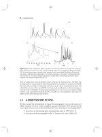
The successful use of HPLC requires an understanding of how separation is affected
by experimental conditions: the column, solvent, temperature, flow rate and so
forth. In this chapter we review some general features of HPLC for use in the
laboratory, in order to develop an adequate separation (method development), to
carry out a routine HPLC procedure for sample analysis, or to solve problems as they
arise. A descriptive or qualitative approach is usually best suited for understanding
both method development and the routine application of HPLC. For this reason
the reader may wish to skim or skip any of the following derivations—at least
initially. Important equations that are useful in practice are enclosed within a box;
for example, Equation (2.5).
2.2 THE CHROMATOGRAPHIC PROCESS
A schematic of an HPLC system is shown in Figure 2.1, with emphasis on the flow
path of the solvent (solid arrows) as it proceeds from the solvent reservoir to the
detector (the solvent is usually referred to as the mobile phase or eluent). A detailed
discussion of each part of the system (HPLC equipment) is given in Chapter 3. After
injection of the sample, a separation takes place within the column, and separated
sample components leave (are eluted or washed from) the column—with detection
in most cases by either ultraviolet absorption (UV) or mass spectrometry (MS); see
Chapter 4 for details on the use of these and other HPLC detectors. The fundamental
nature or ‘‘mode’’ of the separation is determined mainly by the choice of column, as

summarized in Table 2.1. For sample analysis, the predominant HPLC mode in use
today is reversed-phase chromatography (RPC), which features a nonpolar column
in combination with a (polar) mixture of water plus an organic solvent as mobile
phase. Unless noted otherwise, RPC separation will be assumed in this book. Other
HPLC modes are described in later sections of the book, as noted in Table 2.1. In
Chapters 2 through 8 we will assume that the composition of the solvent remains
the same throughout separation, which is called isocratic elution, as opposed to
Samples
Column Detecto
r
Pump
Injection
valve
Solvent
reservoir
Figure 2.1 Schematic of an HPLC system.
2.2 THE CHROMATOGRAPHIC PROCESS 21
gradient elution where the solvent composition is deliberately changed during the
separation (Section 2.7.2, Chapter 9).
The column consists of a cylindrical tube that is typically filled with small
(usually 1.5- to 5-μm diameter) spherical particles (Fig. 2.2a). These particles are
in most cases porous silica, with an individual pore portrayed in Figure 2.2b
as a cylinder of some specified diameter (typically about 10 nm for use with
‘‘small-molecule’’ samples i.e., molecular weights <1000 Da). The inside of each
pore is covered with the stationary phase—in this example, C
18
groups that are
attached to the silica particle. Figure 2.2c shows a more realistic representation of
present-day porous particles for HPLC. The particle is formed by aggregating small,
spherical, subparticles as shown. The actual pores are formed by the spaces between

the subparticles. Because almost all of the surface of the particle is contained within
these pores, most sample molecules are held inside the particle rather than on the
surface of the particle. That is, the internal surfaces of the pores account for 99%
of the total surface area of the particle; the external surface area (and its effect on
separation) is in most cases negligible. The mobile phase surrounds each particle as
(a)
(b)
(c)
Column, showing mobile-phase flow
inlet outlet
mobile
phase
pore
Particle and surrounding mobile phase
stationary
phase
C
18
C
18
C
18
C
18
C
18
C
18
mobile phase
× 10

Porous particle (detail)
particle
Figure 2.2 The HPLC column. (a) Column packed with spherical particles; (b) schematic of
an individual particle, showing an idealized pore with attached C
18
groups; (c) more realistic
picture of a spherical, porous particle, showing detail (10× expansion).
22 BASIC CONCEPTS AND THE CONTROL OF SEPARATION
Table 2.1
HPLC Separation Modes
Chromatographic Mode Comment Details In
Reversed-phase
chromatography (RPC)
The column is nonpolar (e.g., C
18
), and the
mobile phase is a polar mixture of water
plus organic solvent (e.g., acetonitrile);
RPC is the most widely used mode,
especially for water-soluble samples.
Chapter 6, Section
7.3
Normal-phase
chromatography (NPC)
The column is polar (e.g., unbonded silica),
and the mobile phase is a mixture of
less-polar organic solvents (e.g., hexane
plus methylene chloride); NPC is used
mainly for water-insoluble samples,
preparative HPLC, and the separation of

isomers.
Chapter 8
Non-aqueous
reversed-phase
chromatography
(NARP)
The column is nonpolar (e.g., C
18
), and the
mobile phase is a mixture of organic
solvents (e.g., acetonitrile plus methylene
chloride); NARP is used for very
hydrophobic, water-insoluble samples.
Section 6.5
Hydrophilic interaction
chromatography
(HILIC)
The column is polar (e.g., silica or
amide-bonded phase), and the mobile
phase is a mixture of water plus organic
(e.g., acetonitrile); HILIC is useful for
samples that are highly polar and therefore
poorly retained in RPC.
Section 8.6
Ion-exchange
chromatography (IEC)
The column contains charged groups that can
bind sample ions of opposite charge, and
the mobile phase is usually an aqueous
solution of a salt plus buffer; IEC is useful

for separating ionizable samples such as
acids or bases, and especially for the
separation of large biomolecules (e.g.,
proteins and nucleic acids).
Sections 7.5, 13.4.2
Ion-pair chromatography
(IPC)
RPC conditions are used, except that an
ion-pair reagent is added to the mobile
phase for interaction with sample ions of
opposite charge; IPC is useful for the
separation of acids or bases that are weakly
retained in RPC.
Section 7.4
Size-exclusion
chromatography (SEC)
An inert column is used with either an
aqueous or organic mobile phase; SEC
provides separation on the basis of
molecular weight and is used mainly for
large biomolecules or synthetic polymers.
Section 13.8
2.2 THE CHROMATOGRAPHIC PROCESS 23
it flows through the column, and sample molecules can enter the particle pores by
diffusion (there is normally no significant flow of mobile phase through the particle).
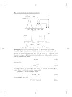
Figure 2.3 illustrates a hypothetical separation of a sample that contains three
sample compounds (or solutes), with individual sample molecules represented by
•
for solute X,  for solute Y,and for solute Z. For clarity, molecules of
the mobile phase are not shown, and molecules of the solvent that the sample is

dissolved in are portrayed by +. The sample is applied to the column in (Fig. 2.3a)
is carried through the column by the flowing mobile phase in successive stages
(Fig. 2.3b–d), and eventually the sample leaves the column (Fig. 2.3e)toprovidea
plot of detector response versus time (a chromatogram, or record of the separation).
As the separation proceeds in Figure 2.3a–d, molecules of sample components X, Y,
and Z exhibit two characteristic behaviors: differential migration and molecular
spreading. By Figure 2.3d, solutes X, Y,andZ have become separated from each
other within the column.
(e)
(f )
(a)(b)(c)(d )
flow
X
Y
Z
+ + + +
+ + + +
0 1 2 3 4 5 (min)
+
solvent
peak
t
0
t
0
t
R
(X)
k =
01234

5
inlet
outlet
Z
Y
X
+ + + +
+ + + +
sample
solvent
column
Figure 2.3 Illustration of the separation process in HPLC. (a–d) Sequential separation within
the column (i.e., as a function of time); (e) the final chromatogram; (f ) estimating values of
k from the chromatogram (e). Solute molecules X, Y,andZ are represented by
•
, ,and,
respectively; sample solvent molecules are shown by +.
24 BASIC CONCEPTS AND THE CONTROL OF SEPARATION
Differential migration (different average speeds at which solute molecules of
X, Y,andZ move, or migrate, through the column) forms the basis of chromato-
graphic separation. Without a difference in migration rates for two compounds,
their separation cannot occur. In this example molecules of X (
•
) move fastest, and
molecules of Z () move slowest; molecules of the sample solvent or mobile phase
are not retained by the column-packing, pass through the column quickest of all,
and leave the column first. Solvent molecules that form part of the injected sample
are represented in Figure 2.3b–e by +.
As a given solute moves through the column, its molecules become increasingly
spread out, so as to occupy a larger volume within the column. The volume that

encompasses the molecules of a given solute within the column defines what is called
a band. The width of this solute-volume is measured in the direction of flow, and
is defined as the band width, as indicated in Figure 2.3a–d for solute X by the
arrow and bracket alongside molecules of X (
•
). When a band leaves the column
and is recorded in the chromatogram (Fig. 2.3e), it is then referred to as a peak.
The identity of each peak can be determined from the time at which it leaves the
column (the retention time t
R
), while the concentration of each solute in the sample
is proportional to peak size (measured either as area or height; see Section 11.2.3).
For sufficiently small samples (low-ng to μg injections, as typically used in HPLC
assay procedures), peak retention times do not change as sample concentration (and
resulting peak size) is varied. In the rest of this chapter we will examine separation
further as a function of experimental conditions.
2.3 RETENTION
The retention time t
R
for each solute is the time from sample injection to the
appearance of the top of the peak in the chromatogram; in Figure 2.3e the retention
times for solutes X, Y,andZ are, respectively, 2, 3, and 5 minutes. The retention
time of the solvent peak at one minute is referred to as the column dead-time t
0
(Section 2.3.1) (sometimes t
m
is used instead of t
0
to represent column dead-time).
The migration rate or velocity u

x
at which solute X moves through the column is
determined by the fraction R of its molecules that are present in the flowing mobile
phase at any time. On average, u
x
will be equal to R times the migration rate or
velocity u of solvent molecules:
u
x
= Ru (2.1)
For example, if half of the molecules of X are in the mobile phase (R = 0.5) and half
are in the stationary phase, only half of the molecules are moving at any given time,
so the average migration rate of X will be one half as fast as that of the solvent.
As illustrated in Figure 2.4, the fraction R of molecules X in the mobile
(moving) phase is determined by an equilibrium process:
X (mobile phase) ⇔ X (stationary phase) (2.2)
Molecules of X in Figure 2.4 are found equally in the mobile and stationary phase
at any time, while molecules of Z predominate in the stationary phase; that is, Z
2.3 RETENTION 25
mobile
phase
stationary
phase
particl
e
XZ
pore
mobile phase
X
Z

Figure 2.4 Equilibrium distribution of solvent and sample molecules between the mobile and
stationary phases, and the resulting effect on solute migration rate. The values of k for solutes
X and Z are 1 and 4, respectively. Equal amounts of X and Z in the sample are assumed.
is more retained than X and therefore migrates more slowly (indicated at the base
of Fig. 2.4 by arrows, whose lengths denote migration rate). This equilibrium and
the migration rate of a given solute are affected by the molecular structure of the
solute, the chemical composition of the mobile and stationary phases (the solvent
and column), and the temperature. The average pressure within the column can have
a small effect on sample retention [1] (see also Section 2.5.3.1), but usually this can
be ignored for moderate pressures (e.g., <5000 psi).
2.3.1 Retention Factor k and Column Dead-Time t
0
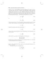
For a given solute, the retention factor k (this is still sometimes referred to as the
capacity factor k

) is defined as the quantity of solute in the stationary phase (s),
divided by the quantity in the mobile phase (m). The quantity of solute in each phase
is equal to its concentration (C
s
or C
m
, resp.) times the volume of the phase (V
s
or
V
m
, resp.), which then gives
k =
C
s

V
s
C
m
V
m
=
C
s
/C
m
V
s
/V
m
= K (2.3)