Introduction to Modern Liquid Chromatography, Third Edition part 8 doc

26 BASIC CONCEPTS AND THE CONTROL OF SEPARATION
where K = (C
s
/C
m
) is the equilibrium constant for Equation (2.2), and  = (V
s
/V
m
)
is the phase ratio—the ratio of stationary and mobile-phase volumes within the
column. We will see that k is a very important property of each peak in the
chromatogram; values of k can help us interpret and improve the quality of a
separation. A solute molecule must be present in either the mobile or stationary
phase so that, if the fraction of molecules in the mobile phase is R, the fraction in
the stationary phase must be 1 − R; therefore from Equation (2.3) we have
k =
1 − R
R
(2.3a)
or
R =
1
1 + k
(2.3b)
The retention time (t
R
)ofX can be defined as distance divided by speed (or band
velocity), where the distance is the column length L and the band velocity is u
x
:

t
R
=
L
u
x
(2.4)
Similarly the retention time of the solvent peak is
t
0
=
L
u
(2.4a)
where u is the average mobile-phase velocity. Eliminating L between Equations (2.4)
and (2.4a)gives
t
R
=
t
0
u
u
x
(2.4b)
which, with R = u
x
/u
0
(Eq. 2.1) and Equation (2.3b), then gives

t
R
= t
0
(1 + k) (2.5)
Equation (2.5) can also be expressed in terms of retention volume V
R
= t
R
F,where
F is the mobile-phase flow rate (mL/min):
V
R
= V
m
(1 + k) (2.5a)
Here V
m
is the column dead-volume, equal to t
0
F (see the further discussion of V
m
and Eq. 2.5a below).
Equation (2.5) can be rearranged to give
k =
t
R
− t
0
t

0
(2.6)
2.3 RETENTION 27
which allows the calculation of values of k for each peak in the chromatogram.
Visual estimates of k from the chromatogram (based on Eq. 2.6) are often used in
practice, because exact values of k are seldom needed for developing a separation
(method development) or during routine analysis. Thus k is equal to the corrected
retention time (t
R
− t
0
), measured in units of t
0
,or
k =

t
R
t
0

− 1 (2.6a)
As illustrated in Figure 2.3f (which corresponds to the chromatogram of Fig. 2.3e),
the distance t
0
can be used to mark off approximate values of k, beginning at time
t
0
; thus k equals 1, 2, and 4, respectively, for compounds X, Y,andZ.
We will see in Section 2.4.1 that values of k between about 1 and 10 are

preferred for various reasons. Therefore it is important to be able to estimate (or
calculate) values of k for the different peaks in a chromatogram, which in turn
requires a value of the column dead-time t
0
. A value of t
0
can often be obtained
from a visual inspection of the initial portion of the chromatogram, as illustrated in
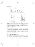
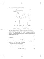
Figure 2.5a–b. Sometimes the first baseline disturbance assumes the characteristic
shape illustrated in Figure 2.5a, which is a clear indication of the unretained solvent
peak. This t
0
-disturbance is usually the result of a change in refractive index (RI)
of the mobile phase (due to differences in RI for the sample solvent vs. the mobile
phase), which in turn affects the amount of light that passes through the flow cell
of the detector. If the sample is dissolved in the mobile phase (usually the preferred
choice), a t
0
peak as in Figure 2.5a may not be observed.
At other times, especially for the injection of a reaction product, environmental
sample, or plant or animal extract, a very large (‘‘excipient’’ or ‘‘junk’’) peak may
be observed at the beginning of the chromatogram (Fig. 2.5b). In this case t
0
corresponds to the initial rise of the peak. Sometimes no obvious solvent peak is
observed (Fig. 2.5c), in which case a value of t
0
can either be measured or estimated.
(a)(b)
t
0

t
0
t
0
t
0
??
(c)(d)
00
00
thiourea
Figure 2.5 Determining the column dead-time t
0
.
28 BASIC CONCEPTS AND THE CONTROL OF SEPARATION
The most direct procedure for determining t
0
is to inject a solute (dissolved in
water or the mobile phase) that is unretained (k = 0) and readily detected, as in
Figure 2.5d. When UV detection below 220 nm is used, thiourea as test solute fulfills
both requirements, and is therefore a good choice for the measurement of t
0
.Other
test solutes have also been used for measuring t
0
, for example, uracil or concentrated
solutions of a UV-absorbing salt such as sodium nitrate [2–4]. Observed values
of t
0
for a given column can vary with mobile-phase composition by as much as

±10–15% for 0–100% B (%B refers to the percent by volume of organic solvent in
the mobile phase), but usually t
0
varies by <5% for 20–80% B [5]. For approximate
estimates of k as in Figure 2.3e, a value of t
0
measured for one value of %B can be
assumed to be the same for all values of %B (when only %B is changed).
Alternatively, a value of t
0
can be estimated from the column dimensions and
flow rate (for columns packed with fully porous particles):
t
0
≈ 5 × 10
−4
Ld
2
c
F
(2.7)
Here L is the column length in mm, d
c
is the column inner diameter in mm, F is
the flow rate in mL/min, and t
0
is in minutes. For several hundred different RPC
columns, it was found that Equation (2.7) agrees with experimental values of t
0
with an average error of only ±10% (1 SD) [6], which again is accurate enough for

practical purposes. The column dead-volume V
m
is related to t
0
as
V
m
= t
0
F ≈ 5 × 10
−4
Ld
2
c
(2.7a)
with L and d
c
in mm. The dead-volume V
m
represents the total volume of mobile
phase inside the column, both inside and outside of the column particles. For
example, if V
m
= 2mL,andF = 0.5mL/min,thent
0
= V
m
/F = 2/0.5 = 4min;t
0
can be regarded as the time required to empty the column of the mobile phase that

was originally present in the column.
For the common case where the column inner diameter ≈ 4.6 mm, we can
conveniently estimate values of V
m
(by combining Eqs. 2.7 and 2.7a):
V
m
(mL) ≈ 0.01L (for 4 to 5 mm i.d. columns, with L in mm) (2.7b)
Values of t
0
can then be obtained from Equation (2.7b), with t
0
= V
m
/F.For
a further discussion of the measurement, accuracy and significance of column
dead-time or dead-volume, see [2–4].
2.3.2 Role of Separation Conditions and Sample Composition
The relative effect of different separation conditions on sample retention k is summa-
rized in the second column of Table 2.2. Table 2.2 is applicable for different HPLC
modes, but the following discussion will assume reversed-phase chromatography
(RPC). The mobile phase for RPC is usually a mixture of water or aqueous buffer
(A-solvent) and an organic solvent (B-solvent) such as acetonitrile or methanol. As
the volume-percent of organic solvent (%B) is increased, the retention of all sample
compounds decreases. A mobile phase that provides smaller values of k is referred to
as a ‘‘stronger’’ mobile phase; similarly water is referred to as a ‘‘weak’’ solvent, and
2.3 RETENTION 29
Table
2.2
Effect of Different Separation Conditions on Retention (k), Selectivity (α), and Plate

Number (N)
Condition k α N
%B ++ + −
B-solvent (acetonitrile, methanol, etc.) + ++ −
Temperature + + +
Column type (C
18
, phenyl, cyano, etc.) + ++ −
Mobile phase pH
a
++ ++ +
Buffer concentration
a
++−
Ion-pair-reagent concentration
a
++ ++ +
Column length 0 0 ++
Particle size 0 0 ++
Flow rate 0 0 +
Pressure −−+
b
Note: ++,majoreffect;+, minor effect; -, relatively small effect; 0, no effect; bolded quantities denote
conditions that are primarily used (and recommended) to control k, α,orN, respectively (e.g., %B is varied
to control korα, column length is varied to control N).
a
For ionizable solutes (acids or bases).
b
Higher pressures allow larger values of N by a proper choice of other conditions; pressure per se, how-
ever, has little direct effect on N (see Sections 2.4.1.1 and 2.5.3.1).

organic solvents are ‘‘strong.’’ Typically values of k decrease by a factor of 2 to 3 for
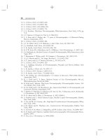
a change of +10% B; an example of the effect of %B on sample retention is shown
in Figure 2.6, for the separation of a mixture of five herbicides. A mobile phase of
80% B in Figure 2.6a results in rapid elution of the sample, with small values of
k (0.3–0.8) and poor separation. When %B is decreased (50% B, Fig. 2.6b), separa-
tion improves, separation or ‘‘run time’’ increases (16 min vs. 1.5 min in Fig. 2.6a),
and peak heights are reduced because the peaks are wider. Retention normally is
controlled within a desired range of k by the choice of %B. The conditions of
Table 2.2 can also be varied in order to control separation selectivity (α) or column
efficiency (N); see Section 2.5 for details.
Reversed-phase chromatography involves a nonpolar stationary phase or col-
umn (e.g., C
18
) and a polar, water-containing mobile phase. Polar solutes will prefer
the polar mobile phase (‘‘like attracts like’’) and be less retained (larger R, smaller
k), while nonpolar solutes will interact preferentially with the nonpolar stationary
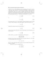
phase and be more retained (smaller R, larger k). The preferential interaction of
a nonpolar solute (n-hexane) with the nonpolar stationary phase is illustrated in
Figure 2.7a, while Figure 2.7b shows the preferential interaction of a polar solute
(1,3-propanediol) with the polar mobile phase. Figure 2.7c is a chromatogram
of several mono-substituted benzenes that vary in polarity or ‘‘hydrophobicity’’
because of the nature of the substituent group. Polar (less hydrophobic) groups such
as –NHCHO, –CH
2
OH, or –OH reduce retention relative to the unsubstituted
solute benzene (shaded peak), while less polar (more hydrophobic) groups such as
chloro, methyl, bromo, iodo, and ethyl increase retention.
30 BASIC CONCEPTS AND THE CONTROL OF SEPARATION
0.2 0.4 0.6 0.8 1.0 1.2 1.4
Time (min)

80% methanol
(0.3 ≤ k ≤ 0.8)
50% methanol
(4 ≤ k ≤ 19)
(a)
(b)
1
2
3
4
5
t
0
51015
1
2
3
4
5
0
Time
(
min
)
Figure 2.6 Separation as a function of mobile phase %B (%v methanol). Herbicide sample:
1, monolinuron; 2, metobromuron; 3, diuron; 4, propazine; 5, chloroxuron. Conditions,
150 × 4.6-mm, 5-μmC
18
column; methanol/water mixtures as mobile phase; 2.0 mL/min;
ambient temperature. Recreated chromatograms from data of [7].

Ionized acids and bases are much more ‘‘polar’’ and therefore less retained than
their neutral counterparts. A change in mobile phase pH that results in increased
solute ionization will therefore lead to a decrease in retention time (Section 7.2).
2.3.2.1 Intermolecular Interactions
This section provides additional insight into sample retention as a function of
the solute, column, and mobile phase; it also represents more information than is
usually required in practice. The reader may therefore prefer to skip to following
Section 2.3.2.2, and return to this section as needed.
The attraction between adjacent molecules of a solute and solvent is the result of
several different intermolecular interactions, as illustrated in Figure 2.8. In principle,
a quantitative understanding of these interactions should allow estimates—or even
predictions—of retention as a function of molecular structure. While this is usually
not possible at the present time (see Section 2.7.7), an understanding of these
interactions can prove useful in other ways; for example, when selecting a different
column for a change in separation (Section 5.4).
Dispersion interactions (Fig. 2.8a) result from the random, instantaneous
positions of electrons around adjacent atoms of either the solvent (S)orthesolute
(X). Typically the arrangement of electrons around the nucleus of atom S will
be unsymmetrical at any instant of time (as in Fig 2.8a), and this will cause the
electrons in adjacent atom X to move as shown (due to coulombic repulsion). The
result is an instantaneous dipole moment for both S and X that favors electrostatic
attraction. The strength of dispersion interactions increases with the polarizability
2.3 RETENTION 31
(a)(b)
sample molecule
H
O H
Nonpolar (hydrophobic) interaction
with the nonpolar stationary phase
Polar(hydrogen bonding)

interaction with the polar
mobile phase
C
18
C
18
C
18
C
18
C
18
C
18
C
18
CH
3
−CH
2
−CH
2
−CH
2
−CH
2
−CH
3
HO−
CH

2
−CH
2
−CH
2
−OH
H
O H
0246
Time (min)
−OCH
3
(anisole)
benzene
−NH−CHO (benzylformamide)
−CH
2
OH (benzyl alcohol)
−OH (phenol)
−CHO (benzaldehyde)
−COCH
3
(acetophenone)
−CN (benzonitrile)
−NO2 −COOCH
3
(methylbenzoate)
−Cl+ −CH
3
(chlorobenzene

+ toluene)
−I
−CH
2
CH
3
−Br
(c)
Figure 2.7 Sample polarity and retention. Illustration of the interaction of a nonpolar sam-
ple solute with the stationary phase (a) and of a polar solute with the mobile phase (b); (c)
effect of different substituents on the retention of monosubstituted benzenes; 150 × 4.6-mm
Hypersil C
18
column, 50% acetonitrile/water as mobile phase, 25
◦
C, 2 mL/min; recreated
chromatogram from data of [8].
of each of the two adjacent atoms. Solute polarizability increases with the size of
the molecule (number of atoms or molecular weight) and with refractive index
[9]; dispersion interactions are therefore stronger for aromatic compounds and for
molecules substituted by atoms of higher atomic weight (sulfur, chlorine, bromine,
etc.)—provided that molecules are of similar size.
Dispersion interactions exist between every adjacent pair of atoms, and this
interaction largely accounts for the physical attraction between molecules of all kinds
(especially for less polar molecules). Because of the nonspecific and universal nature
of dispersion interactions, they are significant in both the mobile and stationary
phases. Dispersion interactions therefore tend to cancel, and they generally play
only a minor role in determining selective interactions of the kind that result
in changes in relative retention when the mobile phase or column is changed.
Dispersion interactions contribute to hydrophobic interactions, so called because

32 BASIC CONCEPTS AND THE CONTROL OF SEPARATION
Dispersion Dipole-dipole
S
X
.
.
.
NO
2
NO
2
Charge transfer (π−π)
(a)(b)
(c)(d)
(e)
CH
3
−C≡N
NO
2
+ − + −
R
N(CH
3
)
2
CH
3
O−H
Hydrogen bonding Ionic

. . .
. . .
O
H−O
+
−
−
+
+−
− +
X
+
Figure 2.8 Intermolecular interactions that can contribute to sample retention and selectivity.
of the attraction of less polar solutes to nonpolar RPC stationary phases (or
their ‘‘water-fearing’’ rejection from the polar aqueous phase). As the strength of
dispersion interactions increases (for larger, less polar solute molecules), the solute
is increasingly retained.
Dipole–dipole interaction is illustrated in Figure 2.8b for the case of dipolar
molecules of solvent (acetonitrile, CH
3
C≡N) and solute (a nitroalkane, R–NO
2
).
The functional groups (–C≡Nand–NO
2
) in these two molecules each have a
large, permanent, dipole moment, causing the two molecules to align for maximum
electrostatic interaction (positive end of one molecule adjacent to the negative
end of the other). The strength of dipole interaction is proportional to the dipole
moments of each of the two interacting groups (not the dipole moment of an entire,

multi-substituted molecule), because dipole interactions are only effective at very
close range (i.e., adjacent atoms or groups).
Hydrogen bonding interactions are shown in Figure 2.8c,fortwocases:
an acidic (or proton-donor) solvent (methanol) interacting with a basic (proton-
acceptor) solute (N,N-dimethylaniline), or an acidic solute (phenol) interacting with
a basic solvent tetrahydrofuran (THF). The strength of hydrogen bonding increases
with increasing hydrogen-bond acidity and basicity of the two interacting species
(Table 2.3).
Ionic (coulombic) interaction is illustrated in Figure 2.8d for a positively
charged sample ion (X
+
) interacting with surrounding molecules of a polarizable
2.3 RETENTION 33
Table
2.3
Solvent Selectivity Characteristics
Normalized Selectivity
a
Solvent H-B Acidity α/ H-B B asicity β/ Dipolarity π
∗
/ P
b
ε
c
Acetic acid 0.54 0.15 0.31 6.0 6.2
Acetonitrile 0.15 0.25 0.60 5.8 37.5
Alkanes 0.00 0.00 0.00 0.1 1.9
Chloroform 0.43 0.00 0.57 4.1 4.8
Dimethylsulfoxide 0.00 0.43 0.57 7.2 4.7
Ethanol 0.39 0.36 0.25 4.3 24.6

Ethylacetate 0.00 0.45 0.55 4.4 6.0
Ethylene chloride 0.00 0.00 1.00 3.5 10.4
Methanol 0.43 0.29 0.28 5.1 32.7
Methylene chloride 0.27 0.00 0.73 3.1 8.9
Methyl-t-butylether 0.00 ≈0.6 ≈0.4 ≈2.4 ≈4
Nitromethane 0.17 0.19 0.64 6.0 35.9
Propanol (n-oriso) 0.36 0.40 0.24 3.9 6.0
Tetrahydrofuran 0.00 0.49 0.51 4.0 7.6
Triethylamine 0.00 0.84 0.16 1.9 2.4
Water 0.43 0.18 0.45 10.2 80
Note: see Appendix I (Table I.4) for additional solvent information.
a
Values from [11], where  refers to the sum of values of α, β,andπ
∗
for each solvent.
b
Polarity index; values from [12].
c
Dielectric constant; values from [13].
solvent. The positive charge on the solute ion causes a displacement of charge in
the solvent molecules, for maximum electrostatic interaction. The strength of ionic
interaction increases for solvents with a larger dielectric constant ε (Table 2.3).
Ionic interaction can also occur between a charged sample ion and ions in either the
mobile or stationary phases; see the discussion of ion-pair chromatography (Section
7.4.1) and ion-exchange chromatography (Section 7.5.1).
Charge transfer or π –π interaction is illustrated in Figure 2.8e for the π -acid
(electron-poor) solute 1,3-dinitrobenzene and the π-base (electron-rich) solvent
benzene. Interactions of this kind can occur between any two aromatic (or unsat-
urated) species, with the strength of the interaction increasing for stronger π-bases
such as polycyclic aromatics (e.g., naphthalene and anthracene), and for stronger

π-acids (e.g., aromatics substituted by electron withdrawing nitro groups). The
solvent acetonitrile (a π-acid) can also interact with aromatic solutes by π –π
interaction [10].
The polar interactions of various nonionic aliphatic solvents used in HPLC can
be described by the solvent-selectivity triangle (Fig. 2.9, [11]). The position of each
solvent in this plot indicates its relative hydrogen-bond acidity α/, hydrogen-bond
basicity β/, and dipolarity π */. Thus amines are relatively strong hydrogen-bond
bases, as indicated by their position near the top of the triangle (large β). Similarly
34 BASIC CONCEPTS AND THE CONTROL OF SEPARATION
H-B Basic
(β/∑)
H−B acidic (α/∑) Dipolar (π∗/∑ )
amines
ethers
THF
DMSO
esters
N,N-dialkyl
amides
ketones
nitriles
nitro compounds
H
2
O
glycols
formamide
alcohols
R-COOH
CH

2
Cl
2
CHCl
3
perfluoroalcohols
basic
solvents
dipolar
solvents
acidic
solvents
Figure 2.9 Solvent-selectivity triangle for aliphatic solvents of various kinds. See Table 2.3 for
values of the solvent properties plotted. Adapted from [11].
nitroalkanes, aliphatic nitriles, and CH
2
Cl
2
all have groups with large dipole
moments, and they are situated near the lower right-hand side of the triangle.
Perfluoroalcohols are especially strong hydrogen-bond donors (and simultaneously
very weak acceptors); they and carboxylic acids (R–COOH) are found near the
lower left of the triangle (large α). Table 2.3 lists (1) relative contributions to solvent
polarity from dipolarity and hydrogen-bond acidity or basicity, (2) a measure of
overall solvent polarity (P

), and (3) values of the dielectric constant ε. Larger values
of ε for the mobile phase indicate increasing ionic interaction with solute molecules
as in Figure 2.8d, increasing solubility in the mobile phase for ionic solutes, and
smaller values of k for ionic solutes. For a comprehensive review of intermolecular

interactions in chromatography, see [14].
More will be said about the solvent-selectivity triangle of Figure 2.9 and solvent
selectivity in Chapters 6 and 8. Section 5.4 on column selectivity provides a similar
treatment of interactions between the solute and the stationary phase.
2.3.2.2 Temperature
Temperature is an important variable in HPLC, as it has a significant effect on
values of k. For most solute molecules and customary separation conditions, solute
retention varies with temperature according to the Van’t Hoff equation, which can
be expressed in HPLC as
log k = A +
B
T
K
(2.8)
2.4 Peak Width and the Column Plate Number N 35
For a given solute and other conditions unchanged, A and B are temperature-
independent constants, and T
K
is the temperature (K). Values of k usually decrease
with increasing temperature (positive value of B)by1–2%per
◦
C; thus a 50
◦
C
increase will cause about a 2-fold decrease in k. As temperature increases, separation
often worsens, while peak heights increase (similar to an increase in %B, as in
Fig. 2.6). It should be noted that deviations from Equation (2.8) are not uncommon,
sometimes resulting in curved plots of log k against 1/T
K
. In a few cases, retention is

observed to increase with an increase in temperature. These exceptions to Equation
(2.8) can arise for various reasons, including changes with temperature of (1) the
ionization of a solute [15, 16], (2) solute molecular conformation [17], and (3) the
stationary phase [18].
Temperature also affects the column plate number N and pressure drop
(see Section 2.4). The practical use of most current HPLC equipment is limited
to temperatures of <80
◦
C (Section 3.7.2), and HPLC column lifetimes often are
shorter at temperatures
>
60
◦
C (Section 5.8). For a further discussion of the role of
temperature in HPLC, see Section 2.5.3.1 and [19–20a].
2.4 PEAK WIDTH AND THE COLUMN PLATE NUMBER N
As illustrated in Figure 2.3, solute molecules spread out to enclose a larger volume
(or form a wider band) during their migration through the column. When the band
leaves the column to become a peak in the chromatogram, it will have a width that
can be defined in various ways. The baseline peak width W is illustrated for the first
peak i of Figure 2.10a. Tangents are drawn to each side of the peak (through the
inflection points), and their intersection with the baseline determines the value of
W. When referring to peak width in this book, we will assume values of baseline
peak width W. The relative ability of a column to furnish narrow peaks is described
as column efficiency, and is defined by the plate number N:
N = 16

t
R
W


2
(2.9)
For example, W for peak i in Figure 2.10a is equal to (4.00 − 3.85) = 0.15 min, and
t
R
= 3.93 min. Therefore N = 16 × (3.93/0.15)
2
= 10, 980. Values of N can vary
for different samples, separation conditions, and columns (Section 2.4.1). The larger
the value of N, the narrower are the peaks in the chromatogram, and the better is
the separation.
Peak width can be measured more conveniently (and precisely) by the
half-height peak width W
1/2
, as illustrated for peak j in Figure 2.10a; values of
W
1/2
≡ 0.588W are reported by many data systems. When the peak width at half
height is used to calculate N,
N = 5.54

t
R
W
1/2

2
(2.9a)