Introduction to Modern Liquid Chromatography, Third Edition part 9 ppt

36 BASIC CONCEPTS AND THE CONTROL OF SEPARATION
(a)
(b)
t
R
(i)
80% B
70% B
0.3 0.8 1.3 (min) 1.0 2.0 (min)
60% B 50% B
2.6 3.1 3.6 (min) 5.8 6.3 6.8 (min)
3.90
4.00 4.10 4.20 4.30
Time (min)
t
R
(j)
i
j
W
W
1/2
h
h/2
3.93 min
1.5
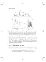
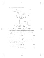
Figure 2.10 Origin and measurement of peak width. (a) Measurement of peak width;
(b) peak 3 of Figure 2.6 as a function of %B, shown with the same time scale for each peak.
Because an ideal chromatographic peak has the shape of a Gaussian curve
(Section 2.4.2), peak width is sometimes described in terms of the standard deviation
σ of the Gaussian curve, where

W = 4σ (2.9b)
and therefore
N =

t
R
σ

2
(2.9c)
Equation (2.9c) can be expressed in other forms, for example, N = 25(t
R
/W
5σ
)
2
,
where W
5σ
= 1.25W is the so-called 5σ peak width.
Equation (2.9) can be rearranged to give
W = 4N
−0.5
t
R
(2.10)
or (replacing t
R
by Eq. 2.5)
W = 4N

−0.5
t
0
(1 + k) (2.10a)
2.4 Peak Width and the Column Plate Number N 37
Because values of N are approximately constant for the different peaks in a
chromatogram, Equation (2.10) tells us that peak width W will increase in proportion
to retention time. A continual increase in peak width from the beginning to the end
of the chromatogram is therefore observed; for example, see the chromatogram of
Figure 2.7c.
The area for a given solute peak normally remains approximately constant
when retention time is varied by a change in %B, temperature, or the column—so
peak height h
p
times peak width W will also be constant. For this situation
h
p
≈
(constant)
W
≈
(constant)
t
R
(2.11)
That is, as t
R
increases, peak height decreases. An example is shown in Figure 2.10b
for peak 3 of Figure 2.6 as a function of %B. A reciprocal change is seen in peak
height and width as %B is varied, as predicted by Equation (2.11).

2.4.1 Dependence of N on Separation Conditions
We will begin by summarizing some practical conclusions about how the column
plate number N varies with the column, the sample, and other separation conditions.
In following Section 2.4.1.1, we will examine the theory on which these conclusions
are based. N can also be described by
N =

1
H

L (2.12)
where H = L/N is the column plate height. H is a measure of column efficiency
per unit length of column; increasing column length (as by replacing a 150-mm
long column with a 250-mm column) is therefore a convenient way of increasing
N and improving separation (since H is constant for columns that differ only in
dimensions).
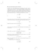
Consider next the log-log plot of Figure 2.11a, which shows how N varies
with flow rate F and particle diameter d
p
(= 2, 5, or 10 μm), while other separation
conditions are held constant. As the mobile-phase flow rate F increases from a
starting value of 0.1 mL/min, N first increases, then decreases. For the present
conditions, maximum values of N (indicated by
•
) are found for flow rates of 0.2
to 1.0 mL/min, depending on particle size d
p
. A 3-fold increase in F,relativeto
the ‘‘optimum’’ value F
opt

for maximum N, has only a minor effect on separation
(a decrease in N of ≈20%) but reduces separation time by 3-fold. Therefore flow
rates greater than F
opt
are usually chosen in practice. Flow rates < F
opt
are highly
undesirable, as this means both lower values of N and longer separation times.
A decrease in particle size generally leads to an increase in N, as seen in
Figure 2.11a. The occurrence of maximum N is seen to occur at higher flow rates for
smaller particles, which allows faster separations for columns packed with smaller
particles (Section 2.4.1.1). The pressure drop across the column (which we will refer
to simply as ‘‘pressure’’ P) increases for smaller particles and higher flow rates (see
the dashed lines in Fig. 2.11a for P = 2000, 5000, and 15,000 psi). The pressure (in
38 BASIC CONCEPTS AND THE CONTROL OF SEPARATION
P (psi) = 2K
5K 15K
10
5
10
4
10
3
10
2
d
p
= 10 μm
0.1 1.0 10 100
F (mL/min)

N
(a)
(b)
150 × 4.6-mm columns
15,000
10,000
5,000
N
0123456
F
(
mL/min
)
80°C,
200 Da
100 × 4.6-mm, 3-μm column
30°C,
6,000 Da
30°C,
200 Da
maximum N
5 μm
2 μm
P (MPa) =
1003414
maximum N
see Section 2.4.1.2
Figure 2.11 Variation of column plate number N with flow rate F, particle diameter d
p
,

and different conditions. Assumes 50% acetonitrile/water mobile phase. (a) Conditions:
150 × 4.6-mm column, 30
◦
C, and a sample molecular weight of 200 Da; (- - -) connects points
on curves of N versus F for pressure P = 2000, 5000, and 15,000 psi, respectively. (b) Con-
ditions: 100 × 4.6-mm column (5-μm particles); other conditions shown in figure. All plots
based on Equation (2.18a) with A = 1, B = 2, and C = 0.05.
psi) for a packed column can be estimated by
P ≈
1.25L
2
η
t
0
d
p
2
(2.13)
or from Equations (2.7) and (2.13),
P ≈
2500LηF
d
p
2
d
c
2
(2.13a)
2.4 Peak Width and the Column Plate Number N 39
Here L is the column length (mm), η is the viscosity of the mobile phase in cP

(see Appendix I for values of η as a function of mobile phase composition and
temperature), t
0
is in minutes, F is the flow rate (mL/min), d
c
is the column internal
diameter (mm), and d
p
is the particle diameter (μm). Other units of pressure (besides
psi) are sometimes used in HPLC: bar ≡ atmospheres = 14.7 psi; megaPascal (MPa)
= 10 bar = 147 psi.
Values of P are also affected somewhat by the nature of the particles within
the column, and how well the column is packed (Section 5.6). Flow restrictions
outside the column (tubing between the pump and detector, sample valve, detector
flow cell) add to the total pressure measured at the pump outlet, but the sum
of these contributions is usually minor (10–20%) compared to values of P from
Equation (2.13)—the exception to this is HPLC systems designed for operation
>
6000 psi with <3-μm particles, which often exhibit a significant pressure in
the absence of a column (e.g., ≥ 1000 psi). Variations in equipment and column
permeability can cause Equations (2.13) and (2.13a) to be in error by ±20% or
more. Despite the ability of most HPLC systems to operate at 5000 to 6000 psi,
it may be desirable to limit the column pressure drop to no more than 3000 psi
(Section 3.5). As the pressure typically increases when a column ages, this suggests
that the pressure for a routine assay with a new column should not exceed 2000 psi.
The latter recommendation is conservative, however, and HPLC systems are now
commercially available for routine use at pressures of 10,000 to 15,000 psi or higher
(Section 3.5.4.3; [21]).
Next consider Figure 2.11b, for a 100 × 4.6-mm column of 5-μm particles,
with a mobile phase of 50% acetonitrile/water (note the linear–linear scale and the

narrower, more typical range in values of F). Plots of N versus flow rate are shown for
three different conditions: 30
◦
C and a 200-Da sample, 30
◦
C and a 6000-Da sample
(e.g., a large peptide), or 80
◦
C and a 200-Da sample. Similar plots of N versus F are
observed for each of these three examples, except that the flow rate for maximum
or optimum N (F
opt
) is shifted to higher values for higher temperatures, and lower
values for larger sample molecules. One conclusion from Figure 2.11b is that higher
flow rates can be used with separations carried out at higher temperatures, which
can in turn be used for faster separations (Section 2.5.3.1). Similarly separations of
higher molecular-weight samples will generally require lower flow rates (and longer
run times) for comparable values of N (e.g., Table 13.4). The dependence of N
on the column, sample molecular weight, and other conditions is summarized in
Table 2.4.
2.4.1.1 Band-Broadening Processes That Determine Values of N
The width W and retention time t
R
of a peak determine the value of N for the
column (Eq. 2.9). Various processes within and outside the column contribute to
the final peak volume or width W, as illustrated in Figure 2.12 (note the increases
in band width that result for each process [Fig. 2.12a–e], indicated by a bracket
plus arrow alongside the band). Following sample injection, but before the sample
enters the column, molecules of a solute will occupy a volume that is usually small
(Section 2.6.1 ). This is illustrated in Figure 2.12a, where individual solute molecules

are represented by
•
. Often the extra-column contribution to band width can be
ignored (Section 3.9), but that depends on the characteristics of the equipment
40 BASIC CONCEPTS AND THE CONTROL OF SEPARATION
Table 2.4
Effect of Different Experimental Conditions on Values of the Plate Number N
Effect on F
opt
, the Value of Effect on N and P of an Increase
Condition F for Maximum N in Specified Condition
a
Column length L None N increases proportionately
P increases proportionately
Column diameter d
c
F
opt
∝ d
c
2
None, if flow rate increased in
proportion to d
c
2
(recommended)
Column particle size
d
p
F

opt
∝ 1/d
p
N decreases (Fig. 2.12)
P decreases
Mobile-phase flow
rate F
None N decreases (Fig. 2.12)
P increases proportionately
Mobile-phase viscosity
η
F
opt
decreases as η increases N decreases (Eqn. 2.19)
P increases proportionately
Temperature T(K) F
opt
increases as T increases
b
N increases (Fig. 2.13c)
P decreases
Sample molecular
weight M
F
opt
∝ M
−0.6
N decreases (Fig. 2.13c) no effect
on P
Note: See discussion of Figures 2.12 and 2.13.

a
Assumes flow rates equal or exceed the optimum value for maximum N (F
opt
), as is often the case.
b
Due to an increase in both T and mobile phase viscosity (Eq. 2.19).
and the size of the column (small-volume columns packed with small particles are
especially prone to extra-column band broadening). Consider next the longitudinal
diffusion of solute molecules along the column, as illustrated in Figure 2.12b.This
process causes band width to increase with time, and it occurs whether or not the
mobile phase is flowing. The time spent by the band during its passage through the
column varies inversely with the flow rate, so the contribution to band width from
longitudinal diffusion decreases for faster flow.
Eddy diffusion represents another contribution to band broadening
(Fig. 2.12c). As molecules of the sample are carried through the column in different
flow streams (arrows) between particles, molecules in slow-moving (constricted
or narrow) streams lag behind, while molecules in fast-moving (wide) streams are
carried ahead. This contribution to band broadening is approximately independent
of flow rate, and depends only on the arrangement and sizes of particles within
the column; band broadening due to eddy diffusion increases for poorly packed
columns. Mobile-phase mass transfer (Fig. 2.12d) is the result of a faster flow of the
stream center (much like the middle of a river). As flow rate increases, the center of
the stream moves relatively faster, and band broadening increases.
A final contribution to band broadening within the column is stationary-phase
mass transfer (Fig. 2.12e). Some sample molecules will penetrate further into a
particle pore (by diffusion) and spend a longer time before leaving the particle
(e.g., molecule i in Fig. 2.12e). During this time other molecules (e.g., j) will have
moved a shorter distance into the particle and spent less time before leaving the
particle. Molecules (e.g., j) that spend less time in the particle will move further
2.4 Peak Width and the Column Plate Number N 41

(j)
(i)
1
2
3
4
5
6
8
7
9
Sample injection
(extra-column band broadening)
Longitudinal diffusion
(time dependent)
(a)(b)
(c)(d)
Eddy diffusion
(flow independent)
Mobile-phase mass transfer
(flow dependent)
Stationary-phase mass transfer
(flow dependent)
Flow through detector +
connecting tubing
(extra-column peak broadenin
g
)
(e)(f )
1

2
3
4
5
6
7
9
8
2
3
1
2
3
4
5
6
8
7
9
Detector
particle
pore
Figure 2.12 Illustration of various contributions to band broadening during HPLC separa-
tion. Molecules of a solute represented by
◦
(before migration) and
•
(after migration); - - -
>
indicates movement of a solute molecule.

along the column, with a consequent increase in band width. This contribution to
band broadening increases as the flow rate increases. Eventually the band leaves the
column and passes through the detector (Fig. 2.12f), resulting in some additional
extra-column peak broadening—as during introduction of the sample to the column
(Fig. 2.12a).
42 BASIC CONCEPTS AND THE CONTROL OF SEPARATION
Band-broadening processes as in Figure 2.12 contribute to the final peak width
W as
W
2
=

W
i
2
(2.14)
where W
i
is the contribution of each (independent) process i to the final peak width.
We can distinguish peak-width contributions that arise either inside or outside of the
column. Let W
EC
represent the sum of extra-column contributions (as in Fig. 2.12a
plus f ), and let W
0
indicate the sum of intra-column contributions so that
W
2
= W
0

2
+ W
2
EC
(2.14a)
The extra-column peak broadening W
EC
should be relatively minor in a well-
designed HPLC system (Section 3.9), so it will be ignored during the following
discussion. Because W
EC
does not depend on values of k, while W
0
(defined by
Eq. 2.10a) increases with k, extra-column band broadening has its largest effect on
early peaks in the chromatogram.
The remainder of this section and Section 2.4.1.2 can be useful for insight
into the dependence of N on experimental conditions. This discussion also provides
a basis for achieving very fast separations (Section 2.5.3.2) and for otherwise
optimizing column efficiency and separation. This material is less essential for the
everyday use of HPLC separation, however, and can be somewhat challenging. The
reader may therefore wish to skip to Section 2.4.2, and return to Section 2.4.1.1
and 2.4.1.2 at a later time. Nevertheless, the material beginning with Equation (2.17)
and especially Section 2.4.1.2 can have great practical value and is very much worth
the reader’s attention. See also the expanded discussion of band-broadening theory
in [22–25].
The quantity W
0
will henceforth be considered equivalent to the peak width
W (Eq. 2.10), which can be expressed in terms of Equation (2.14) as

W
2
= W
2
L
+ W
2
E
+ W
2
MP
+ W
2
SP
longitudinal eddy mobile-phase stationary-phase
diffusion diffusion mass transfer mass transfer
A combination of Equations (2.10) and (2.12) yields
W
2
=

16
L

t
2
R

H (2.15a)
where values of H = L/N for different solutes are approximately independent

of retention time t
R
for a given column of length L and the same experimental
conditions. Therefore
W
2
≈ (constant) H (2.15b)
Equation (2.15) can be more directly related to values of N by replacing values of
W
2
with values of H (Eq. 2.15b):
H = H
L
+ H
E
+ H
MP
+ H
SP
(2.16)
2.4 Peak Width and the Column Plate Number N 43
The quantities H
L,
H
E
, H
MP
,andH
SP
have the same significance as corresponding

values of W in Equation (2.15); H
L
is the contribution to H by longitudinal diffusion,
and so forth. Recalling our discussion above of Figure 2.12, and noting that values
of W
2
are proportional to values of H (Eq. 2.15b), the following expression can be
derived from theoretical equations for each of the four contributions to W:
H = A +
B
F
+ CF
eddy longitudinal mobile-phase plus
diffusion mass transfer stationary-phase mass transfer
where the coefficients A, B,andC are each constant for a particular solute, column,
and set of experimental conditions. If values of F in Equation (2.16a) are replaced
by the mobile-phase velocity u, the so-called van Deemter equation results:
H = A +
B
u
+ Cu (2.16b)
where A, B,andC represent a different set of constants for a particular solute,
column, and set of experimental conditions.
Equation (2.16a) is not quite correct, however, because it assumes that all four
contributions to W are independent of each other. This is not the case for eddy
diffusion and mobile-phase mass transfer; whenever two inter-particle flow streams
combine, remixing occurs, with loss of the velocity profile created by mobile-phase
mass transfer (so-called coupling). We must therefore treat these two processes
(eddy diffusion and mobile-phase mass transfer) as a single band-broadening event.
Because eddy diffusion does not vary with flow rate (∝ F

0
), while mobile-phase mass
transfer does (∝ F
1
), the combination of the two contributions to band width will
vary with some fractional power of F(F
n
). Experimental studies suggest a dependence
of the combined value of H for eddy diffusion plus mobile-phase mass transfer to
the
1
/
3
flow rate power, which leads to an equation of the form
H =
B
F
+ AF
1/3
+ CF
longitudinal eddy diffusion + mobile- stationary-phase
diffusion phase mass transfer mass transfer
(A, B,andC are still another set of constants). A final, generalized relationship
between peak width and experimental conditions can be achieved as follows: A, B,
and C of Equation (2.16c) are variously functions of the solute diffusion coefficient
D
m
and/or particle diameter d
p
, such that Equation (2.16) can be restated as the

so-called Knox equation [25]:
h = Aν
0.33
+
B
ν
+ Cν
(2.17)
Values of the coefficients of Equation (2.17) can be assumed for an ‘‘average’’
separation: A = 1, B = 2, and C = 0.05 (these are very approximate values that
44 BASIC CONCEPTS AND THE CONTROL OF SEPARATION
vary somewhat with the nature of the column—and how well it is packed—and
with values of k). Here we define a reduced plate height h,
h =
H
d
p
(2.18)
and a reduced velocity ν,
ν =
u
e
d
p
D
m
(2.18a)
where u
e
is the interstitial velocity of the mobile phase, as contrasted with the average

mobile-phase velocity u; cgs units are assumed in Equations (2.18) and (2.18a). The
total porosity of the column (as a fraction of the column volume) is defined as ε
T
,
and is composed of the intra-particle porosity ε
i
, plus the inter-particle porosity ε
e
.
The quantity u
e
is then equal to (ε
T
/ε
e
)u, where the quantity (ε
T
/ε
e
) ≈ 1.6.
The solute diffusion coefficient D
m
(cm
2
/sec) can be approximated by a function
of solute molecular volume (V
A
, in mL), temperature (T, in K), and mobile phase
viscosity (η, in cP) by the Wilke–Chang equation [26]:
D

m
= 7.4 × 10
−8
(ψ
B
M
B
)
0.5
T
ηV
A
0.6
(cm
2
/sec) (2.19)
Here M
B
is the molecular weight of the solvent; the association factor ψ
B
is unity
for most solvents, and greater than one for strongly hydrogen-bonding solvents. For
example, ψ
B
equals 2.6 for water and 1.9 for methanol (a value of ψ
B
≈ 2canbe
assumed for typical RPC conditions). Equation (2.19) is reasonably accurate for
solutes with molecular weights <500 Da, and it can represent a useful approximation
for larger molecules.

The Knox equation (Eq. 2.17) provides a conceptual basis for optimizing
conditions, so as to provide maximum values of N in the shortest possible time;
it also forms the basis of the predictions of Table 2.4 and the calculated plots of
Figure 2.11. That is, it is possible to predict (approximately) how values of N will
change when any experimental condition is changed. The practical application of
Equation (2.17) requires the conversion of values of ν into flow rate. Values of F
can be obtained from values of ν as follows: From Equations (2.4a) and (2.7),
F ≈ 0.0005d
c
2
u (2.20)
where flow rate F is in mL/min, column diameter d
c
is in mm, and mobile-phase
velocity u is in mm/min. Equation (2.18a) for u in mm/min, d
p
in μm, D
m
in cm
2
/
sec, and u
e
= 1.6u becomes
ν =
2.7 × 10
−7
ud
p
D

m
(2.20a)
2.4 Peak Width and the Column Plate Number N 45
Combining Equations (2.20) and (2.20a), we have
ν ≈
5.4 × 10
−4
Fd
p
d
c
2
D
m
(2.20b)
and
F =
1850d
c
2
νD
m
d
p
(2.20c)
Figure 2.13a shows a plot of h versus ν(—) based on Equation (2.17) with
values of A = 1, B = 2, and C = 0.05; this plot is independent of the experimental
conditions listed in Table 2.4, and therefore applies (approximately) for all condi-
tions. A minimum value of h ≡ h
opt

≈ 2 is found in Figure 2.13a, corresponding
to a value of ν ≡ ν
opt
≈ 3 (these ‘‘optimum’’ values of h and ν correspond to
maximum values of N). The solid curve of Figure 2.13a is repeated as the solid curve
of Figure 2.13b, except that reduced velocity ν(the x-axis) has now been replaced
by the flow rate F (for a particular set of conditions: 50% acetonitrile-water, 30
◦
C,
200-Da solute, 4.6-mm diameter column). When any of the conditions of Table 2.4
change for the example of Figure 2.13b, the solid-line plot for 30
◦
C and a 200-Da
solute will be shifted right or left, depending on the effect of the change in condition
on the flow rate for maximum N (F
opt
corresponding to ν
opt
≈ 3). Table 2.4 predicts
that F
opt
will increase for an increase in temperature, which is seen (dotted curve)
in Figure 2.13b. Similarly an increase in sample molecular weight will decrease F
opt
and shift the h–ν plot to the left (also seen in Fig. 2.13b as the dashed curve).
Figure 2.11b can be obtained from Figure 2.13b by changing values of h to N (Eqs.
2.12, 2.18).
The reason for changes in F
opt
with conditions (summarized in Table 2.4) is as

follows: Any change in condition that involves either particle size d
p
or the diffusion
coefficient D
m
will change the value of ν, provided that mobile-phase velocity u (and
flow rate F) are held constant. To maintain the same value of ν
opt
≈ 3 for minimum
h and maximum N, the flow rate must then be changed so as to compensate for the
effect of conditions on ν. For example, an increase in temperature will increase the
diffusion coefficient D
m
(Eq. 2.19) by some factor x, which then results in a decrease
in ν by the same factor (Eq. 2.18a). The flow rate corresponding to F
opt
must
accordingly be increased by the factor x, in order to compensate for the temperature
increase and hold ν = ν
opt
constant.
Also shown in Figure 2.13a are plots of each of the three terms that contribute
to Equation (2.17), with the value of ν for minimum h (and maximum N) shown by
the arrow (h ≈ 2, ν ≈ 3). The original Knox equation (Eq. 2.17) has subsequently
been refined, leading to modified relationships that are claimed to offer greater
accuracy, expanded applicability, and/or greater insight into the basis of column
efficiency [27–32]. Additionally values of both B and C depend on the value of
k for the solute [33, 34] when stationary-phase diffusion is taken into account
[35]. Consequently Equation (2.17) is mainly useful for practical, semi-quantitative
application; it has even been described as a ‘‘merely empirical expression’’ [36]

(we do not agree!). Nevertheless, its simplicity, convenience, and fundamental basis
continue to recommend it as a conceptual tool for everyday practice.