Introduction to Modern Liquid Chromatography, Third Edition part 10 ppt

46 BASIC CONCEPTS AND THE CONTROL OF SEPARATION
8
6
4
2
0.1 1.0 10 100
n (optimum)
B/n
h
An
1/3
Cn
h
(a)
8
6
4
2
0.1 1 10
F (mL/min)
30°C
6,000 Da
80°C
200 Da
30°C
200 Da
h
(b)
n
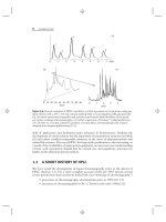
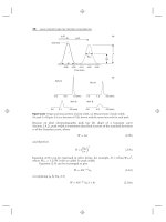
Figure 2.13 Knox equation. (a) Plot of reduced plate height h versus reduced velocity ν with
A = 1, B = 2, and C = 0.05. The total plate height h is shown as a solid curve; the three con-

tributions of Equation (2.17a) to h are shown as dashed or dotted curves. (b) Effect of a change
in solute molecular weight (6000 vs. 200 Da) or temperature (80
◦
Cvs.30
◦
C) on h versus flow
rate. All plots based on Equation (2.17) with A = 1, B = 2, and C = 0.05.
2.4.1.2 Some Guidelines for Selecting Column Conditions
Column conditions can be defined as column length and diameter, particle size, and
flow rate. Together these experimental choices by the user determine the value of
N, run time, and column pressure P. In general, larger values of N require longer
run times, but an increase in the available column pressure can be used to improve
the trade-off between N and run time: either larger values of N for the same run
time or shorter run times for the same value of N. Column diameters can be varied
for different purposes; larger diameters for preparative separations (Chapter 15), or
smaller diameters for (1) increased sensitivity when the amount of sample is limited,
(2) reduced flow rates for LC-MS (Section 4.14), (3) reduced solvent consumption,
2.4 Peak Width and the Column Plate Number N 47
or (4) the use of very high-pressure operation (to minimize problems caused by the
generation of heat within the column; Section 3.5.4.3). Column diameter d
c
does
not directly affect the relationship between N,runtime,andP, but smaller column
diameters mean smaller volume peaks, which are more affected by extra-column
peak broadening; small-diameter columns are therefore more demanding in terms
of equipment. Similarly pressures higher than about 5000 psi also require special
equipment (Section 3.3.5.4) and columns.
Apart from the issue of column diameter, the choice of column conditions can
be guided by the theory of Section 2.4.1.1. The following discussion will assume a
sample molecular weight <1000 Da, but the separation of larger molecules follows

from the discussion of Figure 2.11b and Section 13.3.1. Consider the following three
possibilities:
A. only a single column configuration is available (e.g., a 150 × 4.6-mm
column of 5-μm particles)
B. a single column configuration is available in different column lengths so
that length can be varied
C. there is a wide choice of column lengths and particle size
For case A, only the flow rate can be varied (as in Fig. 2.11a), and there is a
maximum possible flow rate F that is determined by the pressure limit of the system;
however, it is often desirable to operate at a lower pressure. In this situation the
largest value of F should be selected that results in the desired value of N but does
not exceed some maximum pressure. For example, for the 5-μm, 150 × 4.6-mm
column of Figure 2.11a, assume that a value of N ≥ 10,000 is required, while not
exceeding a pressure of 2000 psi. It can be seen(o) that a flow rate of ≈ 2mL/min
will yield a value of N = 10,000, at a pressure <2000 psi.
For case B, both the flow rate and column length L can be varied. Maximum
values of N in minimum time result when the combined choice of values of F and L
results in a maximum column pressure. From Equation (2.13a) this is equivalent to
holding the product FL constant. Figure 2.14a illustrates the resulting dependence
of N on run time (values of t
0
) for three different particle sizes: 2, 5, and 10
μm. A conclusion from Figure 2.14a is that the smallest particles (2 micron) are
preferred for the shortest separation times (and correspondingly for smaller values
of the required N). Thus for a value of t
0
= 1 min, values of N are largest for a
2-μm particle column, while values of N are largest for a 10-μm particle column
when t
0

= 1000 min. Thus, when large values of N are required, larger particles
are best; when small values of N are adequate, smaller particles represent a better
choice because of shorter run times. At intermediate analysis times (e.g., t
0
>
5min),
intermediate-size particles (5 micron) can give the required plate count in less time
than the smallest particles.
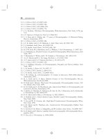
The data of Figure 2.14a are recast into the form of a kinetic or Poppe plot
[37, 38] in Figure 2.14b, where the time required to generate one theoretical plate
(t
0
/N) is plotted against the value of N. This ‘‘time per plate’’ is seen to increase with
the value of N; Figure 2.14b also emphasizes the advantage of small particles when
low values of N are required, and vice versa for large values of N. The dashed lines
labeled ‘‘10 sec,’’ ‘‘100 sec,’’ and ‘‘1000 sec’’ correspond to conditions of constant
t
0
; other values of t
0
are defined by lines parallel to those shown. Poppe plots
48 BASIC CONCEPTS AND THE CONTROL OF SEPARATION
10
6
10
5
10
4
10
3

10
−1
10
−3
10
−2
10
−4
0.1 1 10 1000
N
t
0
(min)
d
p
= 10 mm
(a)
(b)
5 mm
2 mm
5 mm
2 mm
1
t
0
/N (sec)
N
10
6
10

5
10
4
10
3
10
2
d
p
= 10 mm
P = 2000 psi
t
0
= 1000 sec
t
0
= 100 sect
0
= 10 sec
Figure 2.14 Variation of N as a function of column length, holding column pressure constant
by varying flow rate. (a) N versus t
0
for different particle sizes; (b) ‘‘Poppe plot’’ for data of
(a). Calculated values from Equation (2.17), assuming A = 1, B = 2, and C = 0.05, a viscosity
of 0.6 cP (e.g., 60% acetonitrile-water, 35
◦
C), D
m
= 10
−5

cm
2
/ sec (corresponds to a sample
molecular weight of 300 Da for the latter conditions), and a column pressure P = 2000 psi.
are now widely used to compare column performance, as they take both column
efficiency and permeability into account.
For case C, we are permitted to vary column length and particle size contin-
uously. While this will be only approximately true in practice, there is not much
penalty for using column lengths and particle sizes that are not too different from the
optimum. Case C should be considered when the goal is either very fast separation
2.4 Peak Width and the Column Plate Number N 49
or very large values of N (extreme separation conditions). The past decade has
witnessed an increasing demand for faster HPLC separation, sometimes involving
run times of a minute or less (Section 2.5.3.2). Similarly biochemists are now faced
with the need to separate samples that contain thousands of components (Section
13.4.5); in such cases large values of N become more important. Whether the
goal for difficult separations is minimum run time or maximum N, experimental
conditions should be selected that favor maximum N per unit time—as in Figure
2.14b. It can be shown that the best choice of column length, particle size, and
flow rate will always correspond to a minimum value of h ≈ 2(orν ≈ 3). Because
commercial columns are limited to certain lengths and particle sizes, we can only
approximate conditions for ν ≈ 3 while at the same time achieving a required value
of N in the shortest run time. Fortunately, an increase in ν by 2- to 3-fold has only
a small effect on h or N, which gives us considerable flexibility in the selection of a
preferred column length or particle size for a given sample. See also [38a].
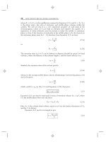
Figure 2.15, which results from the application of Equation (2.17) with ν = 3,
can serve as an example for the selection of conditions that provide maximum N
for a given separation time with some maximum pressure. Assume a maximum
pressure P = 2000 psi, and a value of k = 3 for the last peak in the chromatogram
(for other values of k, adjust the times in Figure 2.15 in accordance with Eq. 2.5).

A value of N = 5000 can be achieved in about 15 sec (marked by
•
and arrow in
the figure). Conversely, N = 300,000 will require about 17 hr (60,000 sec, marked
by
◦
and arrow in the figure). In the first case (N = 5000), ≈1-μm particles will be
required. In the second case (N = 300,000), 9 μm particles are recommended. That
is, fast separations require smaller particles, while large N separations require larger
particles (plus much longer separation times)—as in our preceding discussion of
Figure 2.14. An increase in the allowable pressure results in either shorter times for
the same plate number, or larger values of N for the same time—as the reader can
verify from Figure 2.15 for P = 20,000 compared with 1000 psi. Higher pressures
also favor the use of smaller particles, for either faster separation or larger values of
N. Very large values of N or very short run times require extreme conditions, as can
be inferred from the plot of Figure 2.15.
For various reasons the plots of Figures 2.11 and 2.13 through 2.15 must
be regarded as approximate, as well as varying with other conditions according
to Table 2.4 (e.g., mobile-phase viscosity, sample molecular weight, and tempera-
ture). So these figures should be used primarily as qualitative guides for selecting
experimental conditions rather than quantitative data for a given separation.
Flow rates and column lengths corresponding to Figure 2.15 can be determined
as follows: From Equation (2.18) with H = L/N, and h = 2,
L = NH = Nhd
p
= 2Nd
p
(2.21)
Here cgs units apply: L and d
p

in cm. From Equation (2.18a) for ν ≈ 3,
u =
3D
m
d
p
(2.21a)
50 BASIC CONCEPTS AND THE CONTROL OF SEPARATION
N = 10
6
10
5
10
4
10
3
100
10
1
N = 10
5
N = 2 × 10
4
N = 3 × 10
5
N = 5000
N = 1000
Run time
t (sec)
d

p
= 10 μm
d
p
= 5
d
p
= 1
3
2
1.5
Pressure (psi × 0.001)
1 min
1 hr
0.5 1 2 5 10 20
P = 2000 psi
Figure 2.15 Variation of column plate number N with separation time t, column pressure P,
and particle diameter d
p
. (___) lines representing different values of N; ( ) lines represent-
ing different particle sizes; ( ) line representing a column pressure of 2000 psi. All values
in figure are for minimum plate height, h = 2andk = 3. Adapted from [23] for a viscosity of
0.6 cP (e.g., 60% acetonitrile-water, 35
◦
C) and D
m
= 10
−5
cm
2

/sec (corresponds to a sample
molecular weight of 300 for the latter conditions).
with F given by
F =
3V
m
D
m
Ld
p
(2.21b)
where V
m
is the column dead-volume (equal to t
0
F, Eq. 2.7a). The units of Equation
(2.21b) are mL/sec (F), mL (V
m
), cm
2
/sec(D
m
), cm (L), and cm (d
p
).
2.4.2 Peak Shape
So far we have assumed symmetrical peaks in the final chromatogram. Under ideal
conditions a peak will have a Gaussian shape given by
y = (2π )
−0.5

e
−x
2
/2
(2.22)
2.4 Peak Width and the Column Plate Number N 51
Here x is (t − t
R
)/σ ,wheret is time and σ = W/4; y is the peak height. Actual
peaks in a chromatogram will usually depart slightly from a symmetrical, Gaussian
shape, typically showing more or less tailing as in Figure 2.16a. Peak tailing can
be characterized in either of two ways (Fig. 2.16a): by the asymmetry factor A
s
(left-hand side of figure) or by the tailing factor TF (right-hand side). Values of A
s
and TF are related approximately as
A
s
≈ 1 + 1.5(TF−1) (2.22a)
so that values of A
s
are typically somewhat larger than values of TF (Table 2.5).
Figure 2.16b shows how peak shape varies for different values of A
s
or TF;a
value of A
s
or TF = 1.00 corresponds to a perfectly symmetrical peak. The effect
of peak tailing on the separation of two adjacent peaks in the chromatogram is
illustrated in Figure 2.16c (where only peak tailing varies, as measured by the value

TF =
1.0 1.5 2.0 3.0
A
s
=
1.0 1.7 2.5 4.0
Peak tailing factor TF
= (A + B)/2A (5% values)
(b)
(a)
(c)
TF = 1.0
2.0 3.0
(d )(e)
10% of
peak height
5% of
peak height
AB
Peak asymmetry factor A
s
= B/A (10% values)
t
Figure 2.16 Measurement and effects of peak tailing. (a) Definitions of peak asymmetry and
tailing factors (A
S
and TF); (b) peak shape as a function of asymmetry (A
S
) and tailing (TF)
factors; (c) effect of peak tailing on separation; (d) peak fronting; (e) ‘‘overloaded’’ tailing, in

contrast to ‘‘exponential’’ tailing in (a).
52 BASIC CONCEPTS AND THE CONTROL OF SEPARATION
Table 2.5
Relation of Peak-Tailing and Peak-Asymmetry Factors
Peak-Asymmetry Factor (at 10%) Peak-Tailing Factor (at 5%)
1.0 1.0
1.3 1.2
1.6 1.4
1.9 1.6
2.2 1.8
2.5 2.0
of TF). The two peaks with TF = A
s
= 1.0 are well separated from each other. As
peak tailing increases, however, their separation progressively worsens. Many times
the extent of peak tailing is quite minor (TF < 1.2) and may not be noticed. Tailing
of this magnitude (TF ≤ 1.2) will have a negligible effect on separation, except for
the case of a large peak followed by a very small peak (compare Fig. 2.17d,e).
Less often, peak fronting will be observed (TF < 1.0; Fig. 2.16d), with a similar,
potentially adverse effect on separation. Major peak tailing (TF
>
2) can be highly
detrimental to both separation and quantitative analysis; a common requirement for
routine separations is that TF < 2 for all peaks. Quantitation based on peak area
(Chapter 11) requires integration of the entire peak; this in turn depends on setting
proper integration limits, which can become difficult for the case of severely tailing
peaks.
If peak tailing with TF ≥ 2 is observed, steps should be taken immediately
to correct the problem—whether for a routine assay procedure or during the
development of an HPLC method. The remainder of this book will assume symmetric

peaks, unless noted otherwise. Several possible causes of peak distortion or tailing
exist:
• ‘‘bad’’ column (plugged frit or void; Section 5.8)
• contaminated column (buildup of strongly retained sample contaminants;
Section 5.8)
• column overload (too large a sample; Section 2.6.2)
• a sample solvent that is too strong (Section 2.6.1)
• extra-column peak broadening (Sections 2.4.1, 3.9)
• silanol interactions (including contamination of the column packing by trace
metals; Sections 5.4.4.1, 7.3.4.2)
• inadequate or inappropriate buffering (Section 7.2.1.1)
• use of a higher column temperature with cold (inadequately thermostatted)
mobile phase (Section 2.5.3.1)
See also Section 17.4.5.3. Before attempting to reduce tailing, two kinds of peak
tailing should be distinguished: exponential versus column-overload tailing. Expo-
nential tailing is characterized by a gradual return of the peak to baseline, as in
2.4 Peak Width and the Column Plate Number N 53
R
s
= 1.0
1.5 2.0
1:1
10:1
100:1
1000:1
1000:1
TF = 1.2
1:1000
TF = 1.2
(peaks

reversed)
(a)
(b)
(c)
(d )
(e)
(f )
Figure 2.17 Separation as a function of resolution, relative peak size (1:1. 10:1, etc.), and (e, f )
peak tailing.
Figure 2.16a; column-overload tailing creates a peak with a ‘‘right-triangle’’ appear-
ance, as in Figure 2.16e. A reduction in sample weight will usually reduce the tailing
of an overloaded peak as in Figure 2.16e, while exponential tailing may not change
(or may even increase) when sample size is reduced [39, 40]. Usually it is feasible
(and desirable) to reduce peak tailing so that TF ≤ 1.5.
Various attempts have been made to describe the shape of tailing peaks in
mathematical terms [41, 42], and to define a plate number N that includes the
adverse effect of peak tailing on separation. Values of N for tailing peaks that are
calculated by means of Equation (2.9) (and especially Eq. 2.9a) tend to overstate
column efficiency; actual column performance as measured by the separation of peaks
within the chromatogram usually suggests a lower value of N.TheDorsey–Foley
equation is widely used, in an attempt to correct values of N for peak tailing [43]:
N =
41.7(t
R
/W
0.1
)
2
(B/A) + 1.25
(2.22b)

Here the quantities A and B are defined in Figure 2.16a (at 10% of peak height),
and W
0.1
is the value of W measured at 10% of peak height.
54 BASIC CONCEPTS AND THE CONTROL OF SEPARATION
Still another attempt at a more realistic value of N (taking peak asymmetry
into account) is the so-called 5-σ value:
N = 25

t
R
W
5σ

2
(2.22c)
Here W
5σ
is the peak width measured at 4.5% of peak maximum, similar to the
measurement of N from the width at half height (Eq. 2.9a). The effect of peak tailing
on N becomes more pronounced for peak widths that are measured closer to the
baseline; that is, W
1/2
(least effect) < W < W
5σ
(most effect). Equations (2.22b) and
(2.22c), as well as other expedients [41], provide at best only approximate measures
of column performance for tailing peaks. Peaks that tail cannot be described by
a single generic equation (comparable to Eq. 2.22 for symmetrical peaks), as
witnessed by comparing the two peaks of Figures 2.16a and e; consequently no

single value of N can accurately describe peak width for peaks with TF
>
1.2. For
the characterization of tailing peaks, we recommend a value of N from Equation
(2.9a) together with a value of either A
s
or TF. In many cases peak tailing is tracked
as part of system suitability measurements to assess deterioration of the column; for
such applications nearly any measure of peak tailing will serve to successfully track
changes in peak shape over time.
2.5 RESOLUTION AND METHOD DEVELOPMENT
HPLC method development refers to the selection of separation conditions that
provide an acceptable separation of a given sample; for a more detailed (but less
up-to-date) account than provided by the present book; see [44]. The separation of
two peaks i and j as in Figure 2.10a is usually described in terms of their resolution
R
s
= (difference in retention times)/(average peak width):
R
s
=
2[t
R(j)
− t
R(i)
]
W
i
+ W
j

(2.23)
W
i
and W
j
are the baseline widths W for peaks i and j, respectively. Better
separation (increased resolution) results from a larger difference in peak retention
times and/or narrower peaks. Accurate quantitative analysis based on separations
as in Figure 2.17a is favored by baseline resolution, where the valley between the
two peaks returns to the baseline. For two peaks of similar size (as in Fig. 2.17a),
baseline resolution corresponds to R
s
>
1.5. For preparative separations (Section
15.3.2), baseline resolution also allows a complete recovery of each peak with a
purity of 100%.
Examples of resolution are shown in Figure 2.17 for various values of R
s
(1.0,
1.5, 2.0) and different peak-size ratios ratios (1:1, 10:1, 100:1, 1000:1). As long as
R
s
>
1.5 and the two peaks are symmetrical (TF = 1.0), it is seen that there is little
overlap of the two peaks—regardless of relative peak size. Minor peak tailing as
in Figure 2.17e (TF = 1.2) can lead to a significant loss of resolution when a small
peak follows a large peak, and in such cases a value of R
s
>
2 may be necessary.

2.5 RESOLUTION AND METHOD DEVELOPMENT 55
From a practical standpoint, it is nearly impossible to obtain peaks with TF ≈ 1.0.
Consequently, if a sample component is present in very low concentration, relative
to a closely adjacent major component, it is preferable—if possible—to place the
impurity peak before the main peak, as a means of minimizing the effects of peak
tailing on resolution (compare Fig. 2.17f,e). Changes in relative peak position, so as
to place a smaller peak in front of a larger peak, can sometimes be achieved during
method development by a change in conditions that affect selectivity (Section 2.5.2).
A common goal of HPLC method development is the separation of every peak
of interest from adjacent peaks (with R
s
≥ 2), normally corresponding to a one-third
safety factor (vs. baseline separation with R
s
≈ 1.5, for peaks of comparable size).
The goal of R
s
≥ 2 takes into account minor peak tailing, peaks of moderately
dissimilar size, and the usual slow deterioration of the column over time—with
an increase in both peak width and tailing. Even larger values of R
s
may be
required in some cases. The resolution of two peaks can be improved as described
in Sections 2.5.1 through 2.5.3.
When more than two peaks are to be separated, the goal is usually R
s
≥ 2
for the least well-separated peak-pair. This peak-pair is referred to as the critical
peak-pair, and its resolution is referred to as the critical resolution of the separation;
for example, adjacent peaks 1 and 2 in Figure 2.18a,forwhichR

s
= 0.8, or
in Figure 2.18d,forwhichR
s
= 3.9. Method development usually strives for an
acceptable resolution of the critical peak-pair, which then means an adequate
separation (R
s
≥ 2) for all other peaks as well. In this book, when we refer to the
resolution R
s
of a chromatogram, we mean the critical resolution (unless stated
otherwise).
For method-development purposes, it is convenient to derive an alternative,
approximate expression for resolution from Equations (2.5a) and (2.10a) (assuming
equal widths for the two peaks) [45]:
R
s
=

1
4

k
(1 + k)

(α − 1) N
0.5
(2.24)
(a)(b)(c)

Here resolution is expressed as a function of the retention factor k for the first peak i
(term a), the separation factor α (term b), and column efficiency or the plate number
N (term c). The separation factor α (a measure of so-called separation selectivity or
relative retention) is defined as
α =
k
j
k
i
(2.24a)
The quantities k
i
and k
j
are the values of k for adjacent peaks i and j,as
in Figure 2.10a. For this separation k ≡ k
1
= 1.55, α = 1.12, and N = 11,000;
resolution is therefore given by R
s
= (1/4)(1.55/2.55)(1.12 − 1)(11, 000
0.5
) = 1.9.
Equation (2.24) states that resolution can be improved in any of three different ways
(by varying k, α,orN), but improving separation selectivity (values of α) is by far
the most powerful option.
Equation (2.24) is slightly less accurate than Equation (2.23) but more useful
for interpreting chromatograms during method development. Numerical values of