Introduction to Modern Liquid Chromatography, Third Edition part 11 ppt

56 BASIC CONCEPTS AND THE CONTROL OF SEPARATION
0.2 0.4 0.6 0.8 1.0 1.2 1.4
Time (min)
02
Time (min)
80% methanol
(0.3 ≤ k ≤ 0.8)
70% methanol
(0.8 ≤ k ≤ 2.3)
60% methanol
(1.8 ≤ k ≤ 6.6)
50% methanol
(4 ≤ k ≤ 19)
(a)
(b)
(c)
(d )
1
2
3
4
5
1
2
3
4
5
t
0
0246
Time (min)

1
2
3
4
5
51015
1
2
3
4
5
0
Time (min)
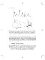
Figure 2.18 Separation as a function of mobile phase %B. Herbicide sample: 1, monolinuron;
2, metobromuron; 3, diuron; 4, propazine; 5, chloroxuron. Conditions, 150 × 4.6-mm, 5-μm
C
18
column; methanol-water mixtures as mobile phase; 2.0 mL/min; ambient temperature.
Recreated chromatograms from data of [7].
R
s
reported in this book are always calculated from Equation (2.23). Equation (2.24)
will be used mainly for an understanding of how resolution depends on various
experimental conditions, and as a guide for systematic method development. An
alternative expression for R
s
in Equation (2.24) is
R
s
=

1
4

k
1 + k

α − 1
α

N
0.5
(2.25)
The derivations of Equations (2.24) and (2.25) are based on different approximations
concerning the widths of the two peaks, and each equation has a similar accuracy.
Equation (2.24) has the advantage of greater simplicity for use in guiding method
development.
The development of an isocratic HPLC method proceeds by systemati-
cally adjusting (‘‘optimizing’’) experimental conditions until adequate separation
is achieved, preferably with a critical resolution R
s
≥ 2. Equation (2.24) provides a
2.5 RESOLUTION AND METHOD DEVELOPMENT 57
useful guide for isocratic method development, as will be explored in Sections 2.5.1
through 2.5.3. Each of terms a–c of Equation (2.24) can be controlled by varying
certain separation conditions (Table 2.2). Usually the first step is to choose a column
with a sufficient plate number that is likely to separate a sample of the required com-
plexity. In many cases, N ≈ 10, 000 is a good starting point, and this can be achieved
either with a 150-mm long column packed with 5-μm particles, or a 100-mm, 3-μm
column. The solvent strength (%B) is next varied to achieve an appropriate range
in values of k (e.g., 1 ≤ k ≤ 10), followed by optimizing selectivity (α). Finally,

the column plate number N can be adjusted for a best compromise between the
conflicting goals of increased resolution vs. a shorter run time.
The final separation conditions we select are hardly ever truly optimum (the best
possible). However, the term ‘‘optimized’’ is often used in the literature to indicate a
relatively improved or preferred separation rather than an absolute best separation.
We should also note the difference between ‘‘local’’ and ‘‘global’’ optimizations.
Local optimization refers to obtaining best values of one or two (seldom more)
separation conditions over a limited range in values of each condition, while other
(usually nonoptimal) conditions are held constant. Global optimization refers to
best-possible values for all conditions that can affect separation or resolution. When
chromatographers report an ‘‘optimized’’ procedure, they almost always are using
this term to describe an improved separation or local optimum. We will continue
this usage in the present book; that is, ‘‘optimum’’ will not be the same as a global
best value of resolution.
2.5.1 Optimizing the Retention Factor k (Term a of Eq. 2.24)
Sample retention k in isocratic elution is usually controlled by varying the
mobile-phase composition (%B). The first step is to achieve values of k for the
sample that are neither too small nor too large. Relative values of resolution R
s
(Eq.
2.24) and peak height h
p
(Eq. 2.11) are plotted against k in Figure 2.19, as a way of
showing how these two quantities vary with k (assuming no change in α with k).
Two peaks at the bottom of Figure 2.19 illustrate how resolution and peak height
change when %B is decreased so as to change the average value of k from 1 to 10.
The usual separation goal is k ≤ 10 for all peaks because this corresponds
to narrower, taller peaks for improved detection, as well as short run times so
that more samples can be analyzed each day. Values of k<<1 can result in poor
resolution, especially from the possible overlap of analytes with matrix interferences

that typically accumulate near t
0
(as in the ‘‘junk’’ peak of Fig. 2.5b). Therefore
1 ≤ k ≤ 10 is usually a goal for all peaks in the final separation (when method
development has been completed). However, at the option of the chromatographer,
it is possible to expand this preferred retention range somewhat, for example, to
0.5 ≤ k ≤ 20. Alternatively, regulatory agencies may recommend k ≥ 2 for all peaks
of interest in the chromatogram [46], in order to minimize possible interference from
sample excipients or other non-assayed (‘‘junk’’) peaks that elute near t
0
. Similarly,
for separation with mass spectrometric detection (LC-MS), it is recommended that
k ≥ 3 because of the possibility of ion-suppression effects. When it is found that
all peaks of interest cannot be accommodated within some maximum range in
k (e.g., 0.5 ≤ k ≤ 20), it is then necessary to use gradient elution (Section 2.7.2,
Chapter 9).
58 BASIC CONCEPTS AND THE CONTROL OF SEPARATION
R
s
, h
p
1.0
0.8
0.6
0.4
0.2
0.0
0246810
k
relative R

s
[k /(1 + k)]
relative peak height h
p
,
[1/(1 + k)]
k = 1
k = 10
Figure 2.19 Relative resolution R
s
andpeakheighth
p
as a function of k orruntime.Runtime
is proportional to the value of 1 + k for the last peak, and α is assumed constant.
The effect of a change in %B on separation is illustrated in Figure 2.18 for RPC.
With 80% methanol/water (80% B) as the mobile phase (Fig. 2.18a), values of k are
small (0.3 ≤ k ≤ 0.8), and as a result the sample is poorly resolved (R
s
= 0.8). With
50% B (Fig. 2.18d;4≤ k ≤ 19), the sample is very well resolved (R
s
= 3.9), but
the run time is longer than necessary, and later peaks are wide (and short)—with
reduced detection sensitivity. An intermediate mobile phase (60% B; Fig. 2.18c)
provides an acceptable range in k (1.8 ≤ k ≤ 6.6) with a reasonable compromise
among resolution (R
s
= 2.6), detection sensitivity, and run time (6 min). A mobile
phase between 60% and 70% B might be an even better choice, offering R
s

>
2.0
with a shorter run time and increased detection sensitivity.
Changes in RPC retention with change in %B (as in Fig. 2.18) can be described
by the empirical relationship [47]
log k = log k
w
− Sφ (2.26)
where φ is the volume fraction of the B-solvent (equal to 0.01 × %B), k
w
is the
extrapolated value of k for solute X with water as the mobile phase (for φ = 0),
and S is a constant for a given compound when only φ is varied. For a review of
the historical development of Equation 2.26, see [48] and references therein. For
‘‘small’’ molecules with molecular weights of 100 to 500 Da, S ≈ 4 [49]. An increase
in φ by 0.1 unit (e.g., a change in the mobile phase by +10% B) will therefore result
in an average decrease in k for all peaks in the sample by a factor of approximately
10
(0.1×4)
, or about 2.5-fold. The latter relationship suggests a systematic procedure
for arriving at a satisfactory value of %B so that 1 ≤ k ≤ 10 (or any other desired
range in k)isachieved.
By this procedure, an initial separation or ‘‘run’’ can be carried out with 80%
or 90% B, which usually ensures that the entire sample will be eluted from the
column in a short time. In the separations of Figure 2.18, for example, the initial
2.5 RESOLUTION AND METHOD DEVELOPMENT 59
run (Fig. 2.18a) with 80% B gives a retention range for the sample of 0.3 ≤ k ≤ 0.8.
Applying the rule of a 2.5-fold increase in k for each 10%B decrease, we can
estimate values of k for lower %B as follows: for 70% B, 2.5 × 0.3 ≈ 0.8for
peak 1 (first peak) and 2.5 × 0.8 ≈ 2.0 for peak 5 (last peak), or 0.8 ≤ k ≤ 2.0.

For 60% B, a similar calculation based on the run with 70% B gives 2.0 ≤ k ≤ 5.
The latter predicted range in k is well within the desired range of 1 ≤ k ≤ 10 (as
is the observed range of 1.8 ≤ k ≤ 6.6); therefore the second method development
experiment should use 60% B as mobile phase (other conditions being the same).
For samples that are much less strongly retained than this sample, the initial
experiment with 80% B might yield k ≈ 0 for all peaks in the chromatogram (i.e.,
a single peak that comprises all of the sample components). In this case a decrease
in %B of at least 30% B will be required for acceptable values of k; the second
experiment might therefore substitute (80–30% B) = 50% B as mobile phase,
followed by further changes in %B for 1 ≤ k ≤ 10—as in the example above based
on Figure 2.18. Because of the approximate nature of the ‘‘rule of 2.5,’’ it is best
not to change %B by
>
30% B between experiments, or late-eluting peaks may
be missed for values of %B that are too low. An alternative (usually preferred)
approach for selecting a suitable value of %B makes use of gradient elution for the
initial experiment in method development (Section 9.3.1).
2.5.2 Optimizing Selectivity α (Term b of Eq. 2.24)
When a further improvement of the separation is needed, relative retention (peak
spacing, selectivity, or separation factor α) is next adjusted by varying any of the
first seven conditions of Table 2.2: %B, the choice of B-solvent (usually methanol
or acetonitrile), temperature, column type, or—for samples that contain acids or
bases—mobile phase pH, buffer concentration, and ion-pair reagent concentration.
Note in Table 2.2 that changes in each of these conditions can also result in changes
in k, so the mobile phase %B may require simultaneous, further adjustment in order
to maintain values of k within an acceptable range in k (usually no greater than
0.5 ≤ k ≤ 20).
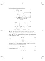
Figure 2.20 provides an illustration of varying selectivity for the separation
of a sample that contains six components. In this example, %B was initially varied
to achieve 2 ≤ k ≤ 4 for the separation of Figure 2.20a. We will further vary %B

and temperature as means for improving selectivity and resolution. For a mobile
phase of 45% B and a temperature of 30
◦
C (Fig. 2.20a), peak-pairs 1–3 and 5/6
are poorly resolved (R
s
= 0.3). A decrease in %B (30% B, Fig. 2.20b)resultsina
better separation of all six peaks, an acceptable retention range (4 ≤ k ≤ 12), but
with marginal resolution of peaks 3 and 4 (which were well resolved in Fig. 2.20a).
A reversal of the positions of peaks 5 and 6 also occurs in Figure 2.20b.Wecan
see from these two chromatograms that an intermediate value of %B is likely to
improve resolution, by moving peaks 3 and 4 apart—before peak-pairs 1/2 or 5/6
come together. In fact a mobile phase of 33% B (and 30
◦
C) for this sample results
in a significant increase in resolution (R
s
= 2.1, not shown).
If temperature is increased from 30 to 45
◦
C (Fig. 2.20c,same%BasFig.2.20a),
further changes in relative retention or selectivity result, but the overall separation is
poor (R
s
= 0.4). If the resolution of this sample is explored further, by trial-and-error
60 BASIC CONCEPTS AND THE CONTROL OF SEPARATION
45% B, 30°C
2 ≤ k ≤ 4,
R
s

= 0.3
30% B, 30°C
4 ≤ k ≤ 12
R
s
= 1.4
45% B, 45
1 ≤ k ≤ 34
R
s
= 0.4
C 20% B, 47
4 ≤ k ≤ 20
R
s
= 4.0
1
024
Time (min)
0246810
Time (min)
1
+
2
+
3
4
6
2
3

4
6
5
1
02
Time
(
min
)
0 2 4 6 8 10121416 18
Time
(
min
)
1
+
2
3
4
5
+
6
2
4
3
6
5
(a)(b)
(c)(d )
t

0
5
C
Figure 2.20 Effect of mobile phase %B and/or temperature on the isocratic separa-
tion of a six-component sample. Sample: 1, 3-phenylpropanol; 2, 1-nitropropane; 3,
oxazepam; 4, p-chlorophenol; 5, eugenol; 6, methylbenzoate. Conditions: mobile phase is
acetonitrile-water; 150 × 4.6-mm C
18
column (5-μm particles); 2.0 mL/min; see figure for
values of %B and temperature (changed conditions bolded in Figs. 2.20b–d). Note that peak
heights are normalized to 100% for tallest peak in each chromatogram. Simulated chro-
matograms based on data of [50, 51].
changes in both %B and temperature, it is possible to achieve a maximum resolution
of R
s
= 4.0 for 20% B and 47
◦
C (Fig. 2.20d), provided that we allow a k-value as
high as 20. The goal of improving selectivity (as in the examples of Fig. 2.20) can be
an increase in resolution, a decrease in run time, or (usually) both. The selection of
conditions for acceptable separation (i.e., method development) should emphasize
changes in selectivity, which can be used for simultaneous improvements in both
resolution and run time. This will be especially true for samples that are more
difficult to separate—those with a large number of components (and a crowded
chromatogram), or peaks with very similar retention (e.g., isomeric compounds).
2.5.2.1 ‘‘Regular’’ and ‘‘Irregular’’ Samples
The present section can be useful as an aid in interpreting separation as a function
of %B (especially in gradient elution). However, this topic is not essential for using
or developing RPC methods. For that reason some readers may prefer to skip to
Section 2.5.3, andreturntothissectionatalatertime.

Samples for reversed-phase separation can be classified as either ‘‘regular’’ or
‘‘irregular’’ [52]. When only %B is varied for a ‘‘regular’’ sample, the chromatogram
appears to expand and contract like an accordion, with little, if any, change in the
spacing of peaks within the chromatogram. The separations of Figure 2.18 provide
a good example for this ‘‘regular’’ sample (a mixture of herbicides). The sample of
Figure 2.20, on the other hand, shows a reversal of retention for peaks 5 and 6
when %B is changed (Fig. 2.20b vs.Fig.2.20a), as well as less pronounced changes
in the relative retention of peaks 1 to 4. This sample can therefore be described as
2.5 RESOLUTION AND METHOD DEVELOPMENT 61
‘‘irregular,’’ in contrast to the ‘‘regular’’ sample of Figure 2.18. A change in %B
affects relative retention (or selectivity) for ‘‘irregular’’ samples but not for ‘‘regular’’
samples. Because of the possibility of peak reversals and peak misidentification for
‘‘irregular’’ samples, peak tracking (Section 2.6.4) becomes more difficult for such
samples.
‘‘Regular’’ samples are usually mixtures of structurally related compounds,
whereas ‘‘irregular’’ samples are mixtures of more dissimilar molecules—as in
Figure 2.20 for this mixture of several compounds of unrelated structure. Never-
theless, predictions of whether a sample is regular or irregular are often uncertain;
experiments where %B is varied as in Figure 2.18 are required for reliable answers
to this question. Regular and irregular samples can also be defined by means of
Equation (2.26). Regular samples will show a strong correlation of values of S and
log k
w
for a given sample (i.e., diverging, near parallel plots), whereas irregular
samples will show a poor correlation (i.e., intersecting plots). Many samples show a
behavior that is intermediate between the examples of Figures 2.18 and 2.20, with
less pronounced changes in relative retention as %B changes. For further informa-
tion concerning regular and irregular retention behavior, see Section 6.3.1 (isocratic
elution) or Section 9.2.3 (gradient elution).
2.5.3 Optimizing the Column Plate Number N (Term c of Eq. 2.24)

2.5.3.1 Effects of Column Conditions on Separation
When selectivity has been adjusted for optimum peak spacing and maximum sample
resolution (Section 2.5.2), an adequate separation will often result. Yet a further
improvement in separation may be possible by varying column conditions (column
length, flow rate, particle size), so as to improve the column plate number N (term c
of Eq. 2.24). Note that relative retention and peak spacing (values of k and α) will
remain the same when only column conditions are changed for isocratic separation;
as a result the optimized peak spacing achieved previously by varying α (term b of
Eq. 2.24) will not be compromised.
An increase in N leads to an increase in resolution (Eq. 2.24), and usually a
longer run time. Conversely, a decrease in N can provide a shorter run time—which
may be of interest when R
s
 2 after optimizing selectivity (see below). Other factors
equal, values of N are proportional to column length (Eq. 2.12) and generally
increase for a decrease in flow rate or particle size. Run time is proportional to t
0
(Eq. 2.5 ) when k does not change, and t
0
is proportional to L/F (Eq. 2.7). Therefore
run time increases proportionately for an increase in column length or a decrease in
flow rate. Similarly the pressure drop P increases for an increase in column length
or flow rate, or a decrease in particle size (Eq. 2.13a). Consequently we need to
balance run time, resolution, and pressure when we vary column conditions in order
to improve separation (Section 2.4.1.2).
As an example of an increase in sample resolution by a change in column
conditions, consider the separation of Figure 2.20b,whereR
s
= 1.4. In the absence
of an improvement in selectivity (as in Fig. 2.20d)—which may not be readily

possible for some samples—an increase in column length can always be used
to increase resolution. Figure 2.21a shows the result of an increase in column
length from 150 mm in Figure 2.20b to 300 mm (e.g., by using two 150-mm
columns connected in series). Baseline separation is now achieved, with R
s
= 1.9.
62 BASIC CONCEPTS AND THE CONTROL OF SEPARATION
010
20
Time (min)
(a)
(b)
(c)
024
Time (min)
0.2 0.4 0.6 0.8
Time (min)
300-mm column, 5-μm particles
2 mL/min, P = 1700 psi
R
s
= 1.9, run time = 20 min
50-mm column, 5-μm particles
3.0 mL/mi, P = 480 psi
R
s
= 2.0, run time = 4 min
30 × 1.0-mm column, 1.5-μm particles
0.5 mL/min, P = 11,000 psi
R

s
= 2.0, run time = 0.7 min
Figure 2.21 Use of a change in column length or flow rate to either increase resolution or
decrease run time. (a) Separation of Figure 2.20b with an increase in column length from 150
to 300 mm, other conditions the same; (b) separation of Figure 2.20d with a decrease in col-
umn length from 150 to 50 mm, and an increase in flow rate from 2.0 to 3.0 mL/min, other
conditions the same; (c)sameas(b) except high-pressure operation and a 30 × 1.0-mm col-
umn with a flow rate of 0.5 mL/min; column conditions are noted in the figure. Simulated
chromatograms based on data of [50, 51].
Although the latter resolution is marginally less than our recommended minimum
value (R
s
≥ 2.0), it should prove acceptable for most applications. The cost of this
increased resolution is a doubling of both run time (to 20 min) and pressure (to
1700 psi). In this example the increase in pressure is acceptable.
When optimizing α as in Section 2.5.2, it is often advisable to strive for excess
resolution, since this can later be traded for a shorter run time, by using a shorter
column and/or a higher flow rate. An example of a change in column conditions that
can reduce run time is provided by the separation of Figure 2.20d,whereR
s
= 4.0.
By shortening the column 3-fold (from 150 to 50 mm) and increasing the flow rate
1.5-fold to 3 mL/min, the run time is decreased 4.5-fold to 4 minutes (Fig. 2.21b).
At the same time the resolution is acceptable (R
s
= 2.0), and so is the pressure
(P = 480 psi). Many samples will have fewer, more widely separated peaks than in
this example, allowing their separation in less than a minute by a suitable choice of
column conditions.
2.5 RESOLUTION AND METHOD DEVELOPMENT 63

In the past many laboratories have preferred columns packed with -5μm
particles. Such columns are less demanding in terms of equipment (Section 3.9), and
are less likely to be plugged by particulates. Today, however, there is increasing use
of columns packed with 3-μm particles or smaller (see following Section 2.5.3.2). If
a change in column conditions is made for either higher resolution or a faster run
time, the same column packing (e.g., Symmetry C18) is strongly recommended,in
order to avoid any change in column selectivity (Section 5.4).
For further details on the choice of column conditions, see Section 2.4.1.2.
2.5.3.2 Fast HPLC
There is increasing emphasis on very fast separations; for instance, with run times
of less than a minute for relatively simple samples (<10–15 components), or a few
minutes for more complex mixtures. Assuming the availability of suitable equipment
and optimized column conditions, the time required by a separation depends on the
value of k for the last peak and the value of α for the least resolved (‘‘critical’’)
peak-pair. Once ‘‘best’’ values of k and α have been established (optimization of
selectivity), resolution and run time depend only on N. Conditions that favor fast
separation include small particles, short columns, and high flow rates.
Further decreases in run time (with no loss in N) can be achieved by one or
more of the following options:
• ultra-high pressure (
>
6000 psi)
• higher temperature
• particles of special design
High-Pressure Operation. It should be clear from Figure 2.15 and the discussion
of Section 2.4.1.1 that a higher pressure can be used to decrease run time, with
no loss in N (or resolution). As in the case of separations at lower pressures,
small particles should be combined with (relatively) short columns and higher flow
rates for fast separation. The use of higher pressures than can be achieved by
conventional HPLC systems (with maximums of 6000 psi or 400 bar) is referred to

as ultra–high-pressure liquid chromatography, or U-HPLC. U-HPLC, with pressures
>
6000 psi can be used for either better resolution (higher values of N) or reduced
run time, as first reported by Rogers [53] and more fully developed by Jorgenson
[54]. Commercial HPLC equipment was later introduced that allows operation at
pressures of 15,000 psi or more.
As an example of how run time can be reduced with the help of high-pressure
operation, Figure 2.21c shows the separation of the sample of Figure 2.20d,usinga
30 × 1.0-mm column, packed with 1.5-μm particles, and a flow rate of 0.5 mL/min;
the resulting pressure is 11,000 psi. A run time of only 0.7 min is achieved (vs.
17 min originally), while maintaining a resolution of R
s
= 2.0. When this result is
compared with the separations of Figs. 2.21a,b, the potential value of higher pressure
operation should be apparent. (Note that some commercial U-HPLC systems are
limited to flow rates of ≤ 5 mL/min, so smaller diameter columns generally are used
to enable high mobile-phase linear velocities for fast separations.) Several similar
examples have been reported [21], where reductions in run time of 2- to 6-fold were
achieved by the use of ultra–high-pressure operation.
64 BASIC CONCEPTS AND THE CONTROL OF SEPARATION
However, it should be noted that certain assumed relationships begin to fail
significantly as the column pressure increases beyond 5000 psi [55]. Mobile-phase
viscosity increases with pressure, so pressure no longer increases proportionately
with flow rate. Values of k and α become pressure dependent [1], and therefore
dependent on column conditions; this is less noticeable at lower pressures. Finally,
heat is generated when a liquid flows through a packed column, and this heat is
proportional to the pressure drop across the column. Changes in temperature within
the column can have adverse consequences on peak shape and plate number [56], as
well as further change values of k and α (undesirable!).
While higher pressure operation has very definite potential advantages,

it requires special equipment (Section 3.5.4.3) and columns (Section 5.6.2).
High-pressure operation has also been claimed to complicate method development
[1, 55]. This is because values of k, diffusion coefficients D
m
, mobile-phase viscosity,
and other properties that affect separation, are more dependent on pressure, which
usually increases during column use (at lower pressures, these properties can be
regarded as essentially independent of pressure). For these and other reasons
(safety, regulatory, cost, and special problems associated with the use of very high
pressures), the extent to which U-HPLC is likely to replace HPLC in the routine
laboratory was not clear at the time this book was published.
High-Temperature Operation. HPLC separation is usually carried out at tem-
peratures between ambient and 50
◦
C. The selection of a specific temperature within
this range is often made on the basis of optimum selectivity (as in the example
of Fig. 2.20d). The use of higher separation temperatures (e.g.,
>
100
◦
C) has been
suggested as a means of shortening run time and improving resolution, as a result
of an increase in N per unit time for a given pressure [57–59]. If we consider
Figure 2.15 again, we recall that run time, the plate number N, and column pressure
are all interrelated. Provided that we select a particle size, column length, and flow
rate for maximum plates per unit time (i.e., ‘‘optimum’’ use of the column, with ν
≈ 3), the value of N increases for higher temperatures. An increase in temperature
results in both a decrease in mobile-phase viscosity (Appendix I) and an increase of
the solute diffusion coefficient D
m

. A lowering of mobile-phase viscosity allows a
higher flow rate for the same pressure (Eq. 2.13a), which is equivalent to an increase
in pressure (as in U-HPLC). An increase in D
m
results in the same value of N at
a higher flow rate and shorter run time (Fig. 2.11b). Consequently an increase in
temperature can, in principle, be used to shorten run time while maintaining the
same value of N—or increase N while maintaining run time the same.
The advantages of high-temperature operation are offset by some correspond-
ing disadvantages. First, HPLC at near-ambient temperatures was often selected in
the past because of a concern that sample degradation might occur during separa-
tion at higher temperature. Although this is a potential complication which many
chromatographers might prefer to avoid, the probability of such sample degradation
is undoubtedly low for most samples [60–62]. A second problem in the use of higher
separation temperatures is the possibility of radial temperature gradients within the
column. Without careful thermostating of both the column and the entering mobile
phase, severe peak distortion can result (Section 3.7.1). Radial temperature gradients
represent a more serious problem when column temperature is increased, although
2.5 RESOLUTION AND METHOD DEVELOPMENT 65
the problem can be minimized by the use of narrower diameter columns that allow
faster equilibration of the column temperature. A third problem is column instability
at higher temperatures, especially for a mobile phase pH outside the range of 2 to
8. Finally, selectivity generally decreases for higher temperatures, although this may
not be true for selected peak-pairs in the chromatogram. The ‘‘best’’ temperature
will often represent a compromise between maximum N and maximum α.
Particles of Special Design. A number of column configurations exist, apart
from the commonly used fully porous particles: columns packed with either pellicular
or shell (superficially porous) particles (Section 5.2.1.1), and monolithic columns
(Section 5.2.4). The relative advantages of each of these different column types will be
discussed (Section 5.2). Pellicular and shell particles can be especially advantageous

for large-molecule separations because of a reduced contribution of the Cν term of
Equation (2.17). Pellicular columns have a thin coating of porous packing material
on a solid bead and are easily overloaded, which restricts their use to very small
samples. Shell columns have a thicker coating of porous packing than pellicular
columns and can be used with sample loadings that are almost as large as those
for fully porous columns. Monolithic columns are much more permeable than
particulate columns, which allows higher flow rates and faster separation, other
factors being equal. The relative merits of these and various conventional columns
can be evaluated by means of Poppe plots as in Figure 2.14b.
2.5.4 Method Development
The preceding discussion of Sections 2.5.1–2.5.3 deals with the selection of experi-
mental conditions for an acceptable HPLC separation, primarily one with baseline
resolution and a reasonable run time. Adequate separation by itself, however, is not
the complete story; other steps are often involved in method development [44]:
• assessment of sample composition and separation goals
• sample pretreatment
• selection of chromatographic mode
• detector selection
• choice of separation conditions
• anticipation, identification, and solution of potential problems
• method validation and the determination of system suitability criteria
Some of these steps may not be required, or they may need only minimal attention.
‘‘Difficult’’ samples and/or demanding assay procedures may involve more than
simply following the steps outlined above and detailed in other chapters of this
book. That is, special problems may arise during method development that require
a logical response, based on the chromatographer’s prior experience and familiarity
with or access to the literature. For some such examples of method development,
see [62, 63].
2.5.4.1 Assessment of Sample Composition and Separation Goals
At the start of method development, available information about the chemical

composition of the sample should be reviewed. If acidic or basic compounds are