Introduction to Modern Liquid Chromatography, Third Edition part 13 ppsx

76 BASIC CONCEPTS AND THE CONTROL OF SEPARATION
Gradient elution refers to a continuous change in the mobile phase during
separation, such that the retention of later peaks is continually reduced; that is, the
mobile phase becomes steadily stronger (%B increases) as the separation proceeds.
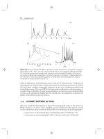
An illustration of the power of gradient elution is shown in Figure 2.25c,where
all peaks for the sample of Figure 2.25a, b are separated to baseline in a total run
time of slightly more than 7 minutes, with approximately constant peak widths and
comparable detection sensitivity for each peak (assuming a similar detector response
for each solute). The advantages of gradient elution for this sample are obvious.
Gradient elution also can be used to deal with several other separation problems, as
discussed in Sections 9.1.1 and 13.4.1.4. For a further discussion of gradient elution,
see Chapter 9.
2.7.3 Peak Capacity and Two-dimensional Separation
So far we have used critical resolution R
s
as the measure of a given separation. This
criterion is appropriate when the peaks of interest in a chromatogram can all be
resolved to some extent, and our goal is some minimum resolution for all peaks.
Some samples contain so many components, however, that it is impractical to achieve
a significant resolution for all peaks of interest. Then we need a different measure of
‘‘separation power’’ for various combinations of experimental conditions. The peak
capacity of a separation refers to the total number of peaks that can be fit into a
chromatogram, when every peak is separated from adjacent peaks with R
s
= 1. An
example is shown in Figure 2.26a, for a retention range of 0 < k ≤ 20 and N = 100.
For isocratic separation, peak capacity is given by [73]
PC = 1 +

N
0.5

4

ln

t
R,z
t
0

= 1 + 0.575N
0.5
log

t
R,z
t
0

(2.30)
where t
R,z
refers to the retention time of the last peak in the chromatogram. For
typical separations, with k ≤ 20 for the last peak and values of N as large as 20,000,
PC = 108. If we exclude peaks with k < 0.5 so that 0.5 ≤ k ≤ 20, the peak capacity
drops to PC = 93; if we require R
s
= 2 the number of peaks that fit between k = 0.5
and 20 drops to 47.
Peak capacity is of much greater importance for separations of complex
samples—those containing a very large number of components. It is seldom possible

to separate such samples with an acceptable resolution of all peaks, so peak capacity
becomes a better measure of overall separation than values of R
s
. Separations of
complex samples are usually carried out by gradient elution, for which the concept
of peak capacity is more relevant (Section 9.3.9.1). Peak capacity is of special interest
for so-called two-dimensional (2D-LC) separation (Section 9.3.10), where fractions
from a first separation are further resolved in a second separation, as illustrated in
the example of Figure 1.4b,c. There it is seen that a group of overlapping peaks from
the first separation (fraction 7) is spread out over the entire chromatogram of the
second separation (orthogonal separation). Under these circumstances the combined
peak capacity for the two separations will be equal to the product of peak capacities
for each separation. For the example above of an isocratic peak capacity of PC
2.7 RELATED TOPICS 77
≈ 100, the 2D-LC peak capacity would be PC = 100 × 100 = 10,000. Thus 2D-LC
separation provides a lot more room in the combined chromatograms for sample
peaks, so it is a powerful technique for separating complex mixtures that contain
hundreds or thousands of individual components.
The peak capacity of a separation should not be confused with the number
of compounds separated at R
s
= 1, since it is rarely possible to achieve a regular
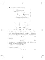
spacing of peaks as in Figure 2.26a [73]. Figure 2.26b illustrates the required
peak capacity PC
req
for the separation (where R
s
≥ 1 for all peaks) of a sample
with n components. Prior to the optimization of selectivity as in Section 2.5.2, a
random arrangement of peaks within the chromatogram can be assumed. As seen in

Figure 2.26b, a sample containing 10 components (‘‘random’’ curve, n = 10) would
require a peak capacity of about 80 to achieve R
s
≥ 1 for every peak. However,
if separation selectivity has been optimized, critical peak-pairs will be separated
to a greater extent, and the required peak capacity would decrease to about 40
(‘‘optimized’’ curve of Fig. 2.26b). See [74] for further details.
2.7.4 Peak Tracking
The interpretation of separations obtained during method development requires
peak tracking or peak matching. For each compound X in the sample, peaks in
0246810
Time (min)
0 ≤ k ≤ 20
peak capacity = 8
(a)
(b)
010203040 50
n
500
400
300
200
100
PC
req
random
ideal spacing (PC
req
= PC)
Required PC (PC

req
) for separation of
n sample components with R
s
= 1.0
“optimized”
Figure 2.26 Peak capacity. (a) Example of peak capacity (PC) for a separation where PC = 8;
N = 100, and R
s
= 1 for every peak; (b) peak capacity required for the separation of a sample
that contains n components [74]; ‘‘ideal spacing’’ is from Equation 2.30.
78 BASIC CONCEPTS AND THE CONTROL OF SEPARATION
the various method development chromatograms that correspond to X must be
characterized or numbered (as in Fig. 2.20). Thus, if peak 1 in run 1 corresponds to
compound A (whose chemical structure may or may not be known), it is necessary to
know which peak in run 2 also corresponds to A. For many samples this may not be
difficult. For example, in Figure 2.20b, d, the six peaks in each run can be matched on
the basis of peak area and relative retention (which usually do not change drastically
when separation conditions are varied). Peaks 3 and 4 change places in these two
chromatograms, but the areas of these and other peaks are sufficiently different to
allow unambiguous peak tracking between the two runs. Manual peak tracking can
take advantage of peak area, peak shape, and the observation that retention order
changes (when they occur) are usually minor (i.e., a peak for a given compound
usually appears in the same region of the chromatogram).
Peak tracking can be much more difficult in other cases, however, for example,
when several peaks overlap as in the two separations of Figure 2.20a,c. While
several workers have suggested ways to improve peak tracking with UV detection
[75–79], no procedure has proved adequate for all samples. Method development
is increasingly making use of mass spectrometer detection (LC-MS), which largely
eliminates problems in peak tracking because of the ability of MS detection to

(1) recognize each of two overlapped peaks and (2) assign a (usually unique)
molecular mass to each peak in the chromatogram [75].
2.7.5 Secondary Equilibria
Chromatographic retention is based on a (primary) equilibrium between a solute
molecule X in the mobile and stationary phases (as in Fig. 2.4 and Eq. 2.2):
X (mobile phase) ⇔ X (stationary phase) (2.2)
Solute molecules may undergo further (secondary) equilibria that involve the ioniza-
tion of acids and bases, ion pairing, complex formation, or isomer interconversion.
As a result it is possible for two forms of the solute to be in equilibrium during their
migration through the column. A common example is the separation of a partially
ionized carboxylic acid, which involves an equilibrium between the ionized and
non-ionized forms:
R−COOH ⇔ R−COO
−
+ H
+
(2.31)
The relative concentrations of each form of the molecule will be determined by
compound acidity (its pK
a
value) and the pH of the mobile phase (Section 7.2),
leading to some fraction F
−
of the molecules being in the ionized form and some
fraction (1 − F
−
) being in the neutral form. If the value of k for the ionized form is
k
−
,andifk

0
refers to k for the non-ionized acid, then a single peak will be observed
for the two species, with its retention given by
k = F
−
k
−
+ (1 − F
−
)k
0
(2.32)
As mobile-phase pH is varied, the ionization of an acidic solute and the value of F
−
will change, as will the value of k (Section 7.2).
2.7 RELATED TOPICS 79
For acid-base equilibria as in Equation (2.31) (for either acidic or basic solutes),
it can be assumed that the ionization process will be quite fast, much faster than
the time required for a solute molecule to move through the column. As a result
each solute molecule will pass back and forth between the ionized and non-ionized
states many times during its migration through the column, and its retention will
be an average value as described by Equation (2.32). Peak width and shape are
not adversely affected by secondary equilibria, despite frequent comments to the
contrary. As noted by McCalley [80], ‘‘the popular assumption that a mixed-mode
mechanism leads inevitably to (peak) tailing is shown to be unfounded.’’ On the
other hand, peak tailing for both acids and bases is sometimes observed, primarily
because of the properties of the column (Section 5.4.4.1) or inadequate buffering of
the mobile phase (Section 7.2.1.1).
When the rate of equilibration between two species is fast, only a single
peak will be observed. This is the case for a partially ionized acid, where the

two forms R–COOH and R–COO
−
rapidly equilibrate during their migration
through the column. When the rate of equilibration between two species is slow,
peak broadening, distortion, and/or the apperance of separate peaks can result.
An example is the interconversion of cis and trans peptide isomers [81]. At higher
temperatures, the interconversion is rapid, and a single, sharp peak is observed
for the peptide where isomerization is possible. At lower temperatures, where the
interconversion is much slower, two distinct peaks are observed. For intermediate
temperatures, a single wide, distorted peak is seen.
2.7.6 Column Switching
Column switching involves the use of two columns connected in a series via a
switching valve (Section 3.6.4.1). A sample is injected into the first column, and
one or more leaving fractions are transferred sequentially to the second column
for further separation. Column switching can be used in each of the following
applications:
• sample preparation (Sections 3.6.4.1, 16.9)
• two-dimensional liquid chromatography (2D-LC) (Sections 9.3.10, 13.4.5,
13.10.4)
• increased sampling rate
The use of column switching for sample preparation or 2D-LC usually involves the
separation of one or more analytes from a complex sample where compounds of
interest are completely overlapped in the first separation (with α ≈ 1.00). To achieve
the separation of compounds with very similar retention, a change in selectivity for
the second separation is usually employed—this is generally achieved by the use
of both a different column and a different mobile phase. An example of such an
application of column switching was illustrated in Figure 1.4b,c.
Another application of column switching for routine analysis can provide
an increase in sampling rate, after conditions have been optimized for the fastest
possible separation. A hypothetical example is illustrated in Figure 2.27a for the

routine assay of peak c or d (or both peaks). The overall run time is 52 minutes,
meaning an assay rate of only slightly more than one sample an hour. Sample
pretreatment in this example might be able to remove late-eluting compounds
80 BASIC CONCEPTS AND THE CONTROL OF SEPARATION
e and f, in which case the separation time could be reduced to about 25 minutes
(a sampling rate of 2.4/hr). If a large number of samples are to be analyzed on a given
day, however, it is possible to significantly increase sampling rate for assays such as
this by means of a column-switching technique called boxcar chromatography [82].
Because the two peaks c and d in Figure 2.27a are well separated from
other peaks in the chromatogram, these two peaks can be segregated from other
sample components with a shorter column and a faster flow rate—as illustrated in
Figure 2.27b for a total run time of < 2 minutes (and a potential assay rate of
>
30
samples/hr). If samples are injected every 2 minutes, a fraction that contains peaks
c and d can be diverted via a switching valve to the column of Figure 2.27a.For
this way of column switching (Fig. 2.27c), a separate pump would deliver the same
mobile phase to the second column at 0.5 mL/min, so as to achieve an equivalent
separation of peaks c and d as in Figure 2.27a (i.e., with adequate resolution).
Because bands c and d occupy only a small fraction of the second column during
their migration through the column, it is possible to simultaneously separate several
samples at the same time, as illustrated in Figure 2.27d. Here 12 fractions from the
first separation can be separated simultaneously, as illustrated by an inside view of
column 2 for fractions 1, 6, 10, and 12 at the beginning of this column-switching
separation (other peaks not shown).
The final separation by the second column is shown in Figure 2.27e; after
a delay of about 25 minutes, separated peaks c and d begin to leave the second
column at a rate of 30 samples per hour. Boxcar chromatography relies on the
simultaneous separation of different samples within column 2, which requires that
two successive samples not overlap during their movement through column 2. To

avoid such sample overlap, the rate of sample injections into column 1 must be
coordinated with the time required for the peaks of interest (e.g., c and d) in a given
sample to leave column 2.
The use of boxcar chromatography has rarely been reported in the literature
[83], and today the availability of mass spectrometric detection might seem to further
reduce the potential advantage of this technique for most samples. Where extremely
large values of N are required for resolution—as in the preparative separation of
compounds differing only in isotopic substitution—boxcar chromatography offers
the possibility of achieving a much higher throughput rate than by any other
technique.
2.7.7 Retention Predictions Based on Solute Structure
Obviously predictions of retention times from experimental conditions and the
molecular structures of sample compounds would be useful for selecting the best
conditions for a separation. Unfortunately, sufficiently accurate predictions of this
kind were generally not possible at the time this book was published. Where
predictions of retention may be useful, however, is for confirmation of the identity
of an unknown peak in the chromatogram. The retention k of a compound is
determined by its molecular structure and separation conditions. For a given set of
conditions, log k can be approximated by
log k = A + R
M(i)
(2.33)
2.7 RELATED TOPICS 81
(a)
(b)
(c)
(d )
(e)
02040
Time (min)

0.2 0.4 0.6 0.8 1.0 1.2 1.4 1.6 1.8
Time (min)
a
b
c
d
e
f
a
b
c
+
d
e
f
column-2
400 × 4.6-mm
3-μm
0.5 mL/min
column-1
50 × 4.6-mm
3-μm
2.0 m/min
waste
detector
column-1
switching valve
column-2
sample
valve

S
S
D
Column switching
1
5
10
15 20
20 30 40 50 60 (min)70
1
6
12
10
Migration through column-2
inlet outlet
Sequential analysis
pump-2
pump-1
Figure 2.27 Illustration of boxcar chromatography for a hypothetical sample. (a) Optimized
separation of the sample for acceptable resolution (column 2); (b) fast separation of the sample
with a shorter column and faster flow rate (column 1); (c) equipment setup for separations of
the present sample by boxcar chromatography; (d) migration of selected sample fractions (1,
6, 10, 12) within column 2, viewed just prior to elution of the fraction for sample 1; (e)early
part of the chromatogram from column 2.
82 BASIC CONCEPTS AND THE CONTROL OF SEPARATION
Here A refers to log k for a parent molecule (e.g., benzene) and R
M(i)
is the
increase in log k that results from the substitution of group i into the molecule
(e.g., insertion of a nitro group i into benzene to form nitrobenzene). Smith [84] has

reported values of R
M(i)
for a number of common substituent groups and different
RPC mobile-phase conditions, allowing estimates of retention as a function of solute
molecular composition (for a very limited number of possible solutes and separation
conditions).
For the case of a homologous series, Equation (2.33) assumes the form
log k = A + nα
CH2
(2.34)
Here n is the number of methylene groups (–CH
2
–) within the molecule, and α
CH2
is the increase in log k due to the addition of one –CH
2
– group to the molecule.
As a consequence of Equation (2.34), plots of log k for a homologous series versus
n are generally observed to be linear (but note the exception of Section 6.2.2
and Fig. 6.5). Relationships similar to Equation (2.34) apply for other compound
series based on the presence of some number n equivalent groups in the molecule
(e.g., oligomers of polyvinylalcohol [–CH
2
CH
2
O– repeating groups], polystyrene
[–CH
2
(C
6

H
5
)CH
2
– repeating groups], etc.) Equations (2.33) and (2.34) are each
referred to as the Martin equation, in recognition of A. J. P. Martin’s first use of
these relationships.
In the case of gradient elution, Equation (2.33) becomes
t
R
≈ A + t
R(i)
(2.35)
where A is the retention time of the parent compound, and t
R(i))
is a constant for
a given group i that is substituted into the parent compound. Equation (2.35) has
been used for the prediction of gradient retention times for a wide variety of solute
molecules; for example, triacylglycerols [85], peptides [86], and polysacchrides [87].
In each case these predictions apply only for a specific set of separation conditions.
While Equation (2.33) or (2.35) can prove occasionally useful in estimating
where a compound peak should be found within a chromatogram, other factors
than the number and kind of substituent groups can have a significant effect on
retention, especially for the complex polar molecules that are commonly present
in samples for HPLC separation. Since the 1950s a large number of workers
have investigated the relationship of sample retention to structure, with the hope
of eventually being able to predict retention and separation in the absence of
experiments (the ‘‘Holy Grail’’ of chromatography). In general, it has not proved
possible to predict chromatographic retention in HPLC with an accuracy that is
anywhere near sufficient to support method development (see [88] for a failed

example). An interesting exception to these past failures of predictions of retention
as a function of solute molecular structure was reported in 2007 [89], where mass
spectrometric detection was combined with retention predictions to permit the
identification of individual peptides in protein-digest mixtures.
2.7.7.1 Solvation-Parameter Model
A well-documented and widely applied solvent-parameter approach has been used
to rationalize RPC retention as a function of the sample, column, and separation
REFERENCES 83
conditions (see [90, 91] and especially [14]). A non-ionized sample is assumed,
in which case retention can be approximated as a result of hydrophobic and
hydrogen-bonding interactions among sample, mobile phase, and column. The
solvent-parameter model takes the form
log k = C
1
+ νV
x
+ rR
2
+ sπ
H
2
+ aα
H
2
+ bβ
2
(2.36)
(i)(ii)(iii)(iv)(v)
A solute retention factor k is related to (1) a constant C
1

that is a function of
column and conditions, (2) solute-dependent quantities ν, r, s, a,andb,and(3)
solute-independent quantities V
x
, R
2
, π
H
2
, α
H
2
,andβ
2
.Termsi to iii of Equation
(2.36) together account for hydrophobic interactions, while terms iv and v are the
result of hydrogen bonding between solute and either the column or the mobile
phase. Values of ν, r, s, a,andb for a large number of different solutes have been
tabulated, and values of C
i
, V
x
, R
2
, π
H
2
, α
H
2

,andβ
2
can be determined for a
column and given conditions by the use of appropriate tests solutes.
Equation (2.36) can provide insight into the factors that determine RPC
separation, but the errors in predictions of values of k (about ±20%) are too large
to be useful for method development. Equation (2.36) is further limited by the fact
that it cannot be applied to ionized solutes, and it neglects a number of additional
interactions that can affect retention (see the related discussion of Section 5.4).
REFERENCES
1. M. M. Fallas, U. D. Neue, M. R. Hadley, and D. V. McCalley, J. Chromatogr. A, 1209
(2008) 195.
2. C. A. Rimmer, C. R. Simmons, and J. G. Dorsey, J. Chromatogr. A, 965 (2002) 219.
3. J. M. Berm
´
udez-Salda
˜
na, L. Escuder-Gilabert, R. M. Villanueva-Cama
˜
nas, M. J. Medina-
Hern
´
andez, and S. Sagrado, J. Chromatogr. A, 1094 (2005) 24.
4. M. Shibukama, Y. Takazawa, and K. Saitoh, Anal. Chem., 79 (2007) 6279.
5. M. A. Quarry, R. L. Grob, and L. R. Snyder, J. Chromatogr., 285 (1984) 19.
6. L. R. Snyder, unreported data. For a single mobile phase (50% acetonitrile/buffer) and
several hundered different columns.
7. T. Braumann, G. Weber, and L. H. Grimme, J. Chromatogr., 261 (1983) 329.
8. L. C. Tan, P. W. Carr, and M. H. Abraham, J. Chromatogr. A, 752 (1996) 1.
9. R. A. Keller, B. L. Karger, and L. R. Snyder, in Gas Chromatography. 1970,R.Stark

and S. G. Perry, eds., Institute of Petroleum, London, 1971, p. 125.
10. K. Croes, A. Steffens, D. H Marchand, and L. R. Snyder, J. Chromatogr. A, 1098 (2005)
123.
11. L.R.Snyder,P.W.Carr,andS.C.Rutan,J. Chromatogr., 656 (1993) 537.
12. L. R. Snyder, J. Chromatogr. Sci., 16 (1978) 223.
13. J. A. Riddick and W. B. Bunger, Organic Solvents, Wiley-Interscience, New York, 1970.
14. M. Vitha and P. W. Carr, J. Chromatogr. A, 1126 (2006) 143.
15. S. M. C. Buckenmaier, D. V. McCalley, and M. R. Euerby, J. Chromatogr. A, 1060
(2004) 117.
84 BASIC CONCEPTS AND THE CONTROL OF SEPARATION
16. S. Heinisch, G. Puy, M P. Barrioulet, and J L. Rocca, J. Chromatogr., 1118 (2006)
234.
17. W. R. Melander, A. Nahum and Cs. Horv
´
ath, J. Chromatogr., 185 (1979) 129.
18. D. Guillarme and S. Heinisch, J. Chromatogr. A, 1052 (2004) 39.
19. J. W. Dolan, J. Chromatogr. A, 965 (2002) 195.
20. G. Vanhoenacker and P. Sandra, J. Sep. Sci., 29 (2006) 1822.
20a. S. Heinisch and J. -L. Rocca, J. Chromatogr. A, 1216 (2009) 642.
21. S. A. C. Wren and P. Tchelitcheff, J. Chromatogr. A, 1119 (2006) 140.
22. J. C. Giddings, Dynamics of Chromatography, Part 1, Principles and Theory, Dekker,
New York, 1965.
23. G. Guiochon, in High-Performance Liquid Chromatography. Advances and Perspec-
tives,Vol.2,C.Horv
´
ath, ed., Academic Press, New York, 1980, p. 1.
24. S. G. Weber and P. W. Carr, in High Performance Liquid Chromatography,P.R.Brown
and R. A. Hartwick, eds., Wiley-Interscience, New York, 1989, p. 1.
25. J. H. Knox, in Advances in Chromatography, Vol. 38, P. R. Brown and E. Grushka,
eds., Dekker, New York, 1998, p. 1.

26. C. R. Wilke and P. Chang, Am. Inst. Chem. Eng. J., 1 (1955) 264.
27. J. H. Knox, J. Chromatogr. A, 960 (2002) 7.
28. L. Kirkup, M. Foot, and M. Mulholland, J. Chromatogr. A, 1030 (2004) 25.
29. F. Gritti and G. Guiochon, Anal. Chem., 78 (2006) 5329.
30. F. Gritti and G. Guiochon, J. Chromatogr. A, 1169 (2007) 125.
31. J. G. Dorsey and P. W. Carr, eds., J. Chromatogr. A, 1126 (2006) 1–128.
32. K. M. Usher, C. R. Simmons, and J. G. Dorsey, J. Chromatogr. A, 1200 (2008) 122.
33. R. W. Stout, J. J. Destefano, and L. R. Snyder, J. Chromatogr., 282 (1983) 263.
34. J. H. Knox and H. P. Scott, J. Chromatogr., 282 (1983) 297.
35. K. Miyabe, J. Chromatogr. A, 1167 (2007) 161.
36. G. Desmet, K. Broekhoven, J. De Smet, S. Deridder, G. V. Baron, and P. Gzil,
J. Chromatogr. A, 1188 (2008) 171.
37. H. Poppe, J. Chromatogr. A, 778 (1997) 3.
38. G. Desmet, D. Clicq, and P. Gzil, Anal.Chem., 77 (2005) 4058.
38a. P. W. Carr, X. Wang, and D. R. Stoll, Anal.Chem., 81 (2009) 5342.
39. D. V. McCalley, J. Chromatogr. A, 793 (1998) 31.
40. D. M. Marchand, L. R. Snyder, and J. W. Dolan, J. Chromatogr. A, 1191 (2008) 2.
41. J. J. Kirkland, W. W. Yau, H. J. Stoklosa, and C. H. Dilks, Jr., J. Chromatogr. Sci.,15
(1977) 303.
42. K. Lan and J. W. Jorgenson, J. Chromatogr. A, 915 (2001) 1.
43. J. P. Foley and J. G. Dorsey, Anal. Chem., 55 (1983) 730.
44. L. R. Snyder, J. J. Kirkland, and J. L. Glajch,
Practical HPLC Method Development,
2nd
ed., Wiley-Interscience, New York, 1997.
45. L. R. Snyder and J. J. Kirkland, Introduction to Modern Liquid Chromatography, 2nd
ed., Wiley-Interscience, New York, 1979, pp. 34–36.
46. Reviewer Guidance. Validation of Chromatographic Methods, Center for Drug Evalu-
ation and Research, Food and Drug Administration (Nov. 1994).
47. K. Valk

´
o, L. R. Snyder and J. L. Glajch, J. Chromatogr., 656 (1993) 501.
48. L. R. Snyder, J. W. Dolan, and J. R. Gant, J. Chromatogr., 165 (1979) 3.
49. L. R. Snyder and J. W. Dolan, J. Chromatogr. A, 721 (1996) 3.
REFERENCES 85
50. N. S. Wilson, M. D. Nelson, J. W. Dolan, L. R. Snyder, R. G. Wolcott, and P. W. Carr,
J. Chromatogr. A, 961 (2002) 171.
51. N. S. Wilson, M. D. Nelson, J. W. Dolan, L. R. Snyder, and P. W. Carr, J. Chromatogr. A,
961 (2002) 195.
52. L. R. Snyder and J. W. Dolan, High-Performance Gradient Elution, Wiley-Interscience,
New York, 2007, ch. 1.
53. B. A. Bidlingmeyer, R. P. Hooker, C. H. Lochmuller, and L. B. Rogers, Sep. Sci.,4
(1969) 439.
54. J. E. MacNair, K. E. Lewis, and J. W. Jorgenson, Anal. Chem., 69 (1997) 983.
55. F. Gritti and G. Guiochon, J. Chromatogr. A, 1187 (2008) 165.
56. R. G. Wolcott, J. W. Dolan, L. R. Snyder, S. R. Bakalyar, M. A. Arnold, and J. A.
Nichols, J. Chromatogr. A, 869 (2000) 211.
57. T. Greibrokk and T. Andersen, J. Chromatogr. A, 1000 (2003) 743.
58. X. Yang, L. Ma and P. W. Carr, J. Chromatogr. A, 1079 (2005) 213.
59. F. Lestremau, A. Cooper, R. Szucs, F. David, and P. Sandra, J. Chromatogr. A, 1109
(2006) 191.
60. F. D. Antia and C. Horv
´
ath, J. Chromatogr., 435 (1988) 1.
61. J. D. Thompson and P. W. Carr, Anal. Chem., 74 (2002) 1017.
62. K. P. Xiao, Y. Xiong, F. Z. Liu, and A. M. Rustum, J. Chromatogr. A, 1163 (2007)
145.
63. L. Deng, H. Nakano, and Y. Wwasaki, J. Chromatogr. A, 1165 (2007) 93.
64. J. C. Sternberg, in Adv. Chromatogr., 2 (1966) 205.
65. M. Tsimidou and R. Macrae, J. Chromatogr. , 285 (1984) 178.

66. N. E. Hoffman, S L. Pan, and A. M. Rustum, J. Chromatogr., 465 (1989) 189.
67. N. E. Hoffman and A. Rahman, J. Chromatogr., 473 (1989) 260.
68. E. Loeser and P. Drumm, J. Sep. Sci., 29 (2006) 2847.
69. E. Loeser, S. Babiak, and P. Drumm, J. Chromatogr. A, 1216 (2009) 3409.
70. H. Colin, M. Martin, and G. Guiochon, J. Chromatogr., 185 (1979) 79.
71. S. R. Bakalyar, C. Phipps, B. Spruce, and K. Olsen, J. Chromatogr. A, 762 (1997) 167.
72. J. E. Eble, R. L. Grob, P. E. Antle, and L. R. Snyder, J. Chromatogr., 405 (1987) 51.
73. J. M. Davis and J. C. Giddings, Anal. Chem. 55 (1983) 418.
74. J. W. Dolan, L. R. Snyder, N, M. Djordjevic, D. W. Hill, L. Van Heukelem, and T. J.
Waeghe, J. Chromatogr. A, 857 (1999) 1.
75. G. Xue, A. D. Bendick, R. Chen, and S. S. Sekulic, J. Chromatogr. A, 1050 (2004) 159.
76. J.L.Glajch,M.A.Quarry,J.F.Vasta,andL.R.Snyder,Anal. Chem., 58 (1986) 280.
77. H. J. Issaq and K. L. McNitt, J. Liq. Chromatogr., 5 (1982) 1771.
78. J. K. Strasters, H. A. H. Billiet, L. de Galan, and B. G. M. Vandeginste, J. Chromatogr.,
499 (1990) 499.
79. E. P. Lankmayr, W. Wegscheider, J. Daniel-Ivad, I. Kolossv
´
ary, G. Csonka, and M.
Otto,
J. Chromatgr.,
485 (1989) 557.
80. D. V. McCalley, Adv. Chromatogr., 46 (2007) 305.
81. W. R. Melander, J. Jacobson and Cs. Horv
´
ath, J. Chromatogr., 234 (1982) 269.
82. L. R. Snyder, J. W. Dolan, and Sj. van der Wal, J. Chromatogr., 203 (1981) 3.
83. A. Nazareth, L. Jaramillo, R. W. Giese, B. L. Karger, and L. R. Snyder, J. Chromatogr.,
309 (1984) 357.
84. R. M. Smith, J. Chromatogr. A, 656 (1993) 381.