Introduction to Modern Liquid Chromatography, Third Edition part 16 pdf

106 EQUIPMENT
ball
flow
seat
(a)
(b)
(c)
seal
seat
piston
spring
piston
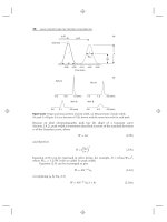
Figure 3.12 Check-valve designs. (a) Simple ball and seat; (b, c) active check valves.
pump head. Ceramic check valves may be used in some pumps, and sometimes a
small spring is used to assist check-valve closure.
Operation of the ball-type check valve is quite simple. When the pressure on
the inlet side of the valve (below the ball in Fig. 3.12a) is higher than that on the
outlet side, the ball will be displaced from the seat and solvent will flow through the
valve. When the pressure is higher on the outlet side (above the ball in Fig. 3.12a),
the ball will be pushed against the seat, which creates a seal so that no liquid
passes through the valve. As described above, and illustrated in Figure 3.11, the inlet
and outlet check valves allow the pump head to alternately fill with mobile phase
from the reservoir and deliver mobile phase to the column. An alternative to the
ball-type check valve is the active check valve, shown in Figure 3.12b and described
in Section 3.5.1.3.
3.5 PUMPING SYSTEMS 107
Time
(a)
(b)
(c)
(d )

Flow
Pressure
Figure 3.13 HPLC pump designs with corresponding flow and pressure profiles.
(a) Single-piston reciprocating pump; (b) effect of a shaped driving cam; (c) dual-piston pump;
(d) accumulator or tandem-piston design.
The single-piston pump with a constant-speed, linear drive will spend half
of the time filling and half of the time delivering solvent. The resulting flow (and
pressure) profile is shown in Figure 3.13a. These extreme pulses in flow and pressure
are undesirable for HPLC applications.
An alternative single-piston design uses a specially shaped (e.g., elliptical)
driving cam on the motor, or a variable-speed, stepper-driven motor, to move the
piston. With this modification, the piston speed can be varied within each pump
cycle so that more than half of the time is spent in the delivery cycle and a small
fraction of the time is spent in the fill cycle (Fig. 3.13b). Some pumps refine this
108 EQUIPMENT
process further so that the pump controller remembers the pressure on the prior
stroke and moves the piston forward rapidly at the beginning of the delivery stroke
until the previous pressure is reached. Then the piston slows to a constant speed
until the end of the delivery stroke. Even with variable-speed design and extensive
pulse dampening, the single-piston pump does not produce a sufficiently stable flow
and pressure for analytical HPLC. Two refinements of the single-piston pump are
the dual-piston pump (Fig. 3.13c, Section 3.5.1.1) and the accumulator-piston pump
(Fig. 3.13d, Section 3.5.1.2).
In addition to the pump components shown in Figure 3.11, most pumps have
a purge valve on the outlet side of the pump that directs the pump output to waste
during pump priming, solvent changeover, and bubble removal. Many pumps also
have a fitting on the inlet side of the pump that allows for manually priming the pump
with the aid of a syringe. In the past, mechanical pulse dampers (e.g., Bourdon tubes)
were used to compensate for pump pulsations; today, the need for mechanical pulse
damping is due to low-pulse pump designs (e.g., dual-piston or accumulator-piston

pumps, Sections 3.5.1.1, 3.5.1.2). Pulse dampers also add unwanted dwell volume
for gradient applications (Section 3.5.3).
3.5.1.1 Dual-Piston Pumps
One way to minimize the pulsations of the single-piston pump is to use two pump
heads in parallel so that, when one is filling, the other is delivering solvent. This is
illustrated in Figure 3.13c with opposing pistons driven off the same cam. Although
most designs use two cams driven off the same motor, the pistons are mounted in
parallel beside each other for operational convenience. With the use of a specially
shaped driving-cam with the dual-piston pump, the pump output can be quite
smooth, requiring little, if any additional pulse dampening. Dual-piston pumps are
one of the two most widely used pump designs for analytical HPLC today.
3.5.1.2 Accumulator-Piston Pumps
An alternative design for the dual-piston pump is the accumulator-piston, or
tandem-piston design shown in Figure 3.13d. In this case, one piston feeds into
the other piston at twice the flow rate. For example, if a flow rate of 1 mL/min was
desired, the top piston (Fig. 3.13d) would pump at 1 mL/min. While the top piston
delivered solvent, the top (outlet) check valve would be open and the intermediate
check valve (inlet for the top piston) would be closed. Meanwhile the lower piston
would fill at a rate of 2 mL/min, with its inlet check valve open. Next, the lower
piston would deliver solvent at 2 mL/min (while the upper piston filled), which
would cause its inlet check valve to close and the intermediate check valve to open.
Half of this 2 mL/min flow (1 mL/min) would be used to fill the top piston and half
would be pumped directly to the column.
The accumulator-piston design, at least in theory, has several advantages over
the dual-piston design. Flow never stops to the column, so flow and pressure pul-
sations should be minimized. Because the check valves can be the most problematic
components in the entire HPLC system, the reduction of the number of check
valves from four (dual-piston) to three (accumulator-piston) can reduce check valve
problems. Furthermore, because solvent is always flowing to the column, the outlet
check valve on the top pump is not necessary and it can be eliminated so that just

3.5 PUMPING SYSTEMS 109
two check valves remain. Although the simplicity of the accumulator-piston design
makes it appear to be more reliable, many other factors go into the final pump per-
formance (software, materials, assembly, mechanical tolerances, etc.). Most workers
obtain comparable performance with either the dual-piston or accumulator-piston
design.
3.5.1.3 Active Check Valve
A final refinement in design can be applied to both the dual-piston and
accumulator-piston pump designs. The ball-type check valve (Fig. 3.12a)is
susceptible to leakage if a tiny bit of debris is lodged between the ball and the
seat. The surfaces are very hard (commonly sapphire and ruby), and even with
the pressure of the pump pushing them closed, the ball-type valve can leak when
particulates are present.
The active check valve is an alternative design that works well as an inlet check
valve on the low-pressure side of the pump. As illustrated in Figure 3.12b, the active
check valve depends on a polymeric seal and a mechanically driven piston to provide
the sealing action. During the fill stroke, the piston is lifted off the seal and solvent
flows into the pump. During the delivery stroke, the piston is pulled against the seal.
The increased surface area relative to the ball-type valve and the soft seal allows
the active check valve to seal effectively, even when a small amount of particulate
matter is present. In an alternative design of the active check valve (Fig. 3.12c), a
ball-type check valve is used with a strong spring to close the check valve; a piston
below the ball pushes it from the seat to open the valve.
In the active check-valve system with dual-piston pumps (Fig. 3.13c), only
two ball-type valves are used (the outlet check valves). With the accumulator-piston
design, only one ball-type valve remains (the check valve between the upper and
lower pump chambers in Fig. 3.13d; the outlet check valve is not needed). In both
cases a reduction in the number of ball-type check valves improves pump reliability.
3.5.2 On-line Mixing
For isocratic methods the mobile phase can be hand-mixed; no additional mixing

is then required within the HPLC system. On the other hand, most users take
advantage of the convenience of on-line mixing and use the HPLC system to blend
the mobile phase for isocratic methods, as well as for gradient methods where
on-line mixing is required. Even when on-line mixing is available, some premixing
of the mobile phase often gives quieter baselines, and in some cases, such as use
with refractive index detection (Section 4.11), on-line mixing is unsuitable for good
baselines at high sensitivity. On-line mixing takes place by one of three techniques:
• high-pressure mixing
• low-pressure mixing
• hybrid systems
3.5.2.1 High-Pressure Mixing
With high-pressure-mixing systems (Fig. 3.14), each solvent is delivered to the mixer
by a dedicated pump. The ratio of solvents in the mobile phase is controlled by the
110 EQUIPMENT
controller
pumps
mixer
dwell-
volume
to
column
injector
A
B
Figure 3.14 HPLC system with high-pressure mixing. Dwell-volume located inside dashed
line.
relative flow rates of the pumps. For example, if 1 mL/min of a 60/40 MeOH/water
mobile phase (60%B) is selected, the MeOH pump delivers 0.6 mL/min and the
water pump delivers 0.4 mL/min. During gradient operation—where %B changes
during the separation—the relative pump speeds change with the gradient program.

Because the solvents are blended under high pressure, outgassing (Section 3.3.1) is
less of a problem than with low-pressure mixing, so degassing problems usually are
minimal. High-pressure-mixing systems are generally limited to the simultaneous
use of two solvents, since another pump is required for each additional solvent.
Some HPLC systems have a solvent-selector valve on one or both pumps that allows
the nonsimultaneous use of two or more solvents by the same pump. This can be
useful for method development (e.g., ACN and MeOH in separate runs) or for
automated system flushing (e.g., flushing with water to remove buffer from the
system). High-pressure mixing systems have an advantage over low-pressure mixing
in that the standard mixer can be replaced with a micro-mixer (Section 3.4.2.3) for
applications, such as LC-MS (Section 4.14), that require minimum dwell-volumes.
Parts of the flow-stream that contribute to system dwell-volume are segregated
within a dashed box in Figs. 3.14 and 3.15 (see also Section 3.5.3).
injector
pump
to
column
dwell-
volume
mixer
solvent
proportioning
valve
controller
B
A
Figure 3.15 HPLC system with low-pressure mixing. Dwell-volume located inside dashed
line.
3.5 PUMPING SYSTEMS 111
3.5.2.2 Low-Pressure Mixing

With low-pressure-mixing systems (Fig. 3.15), the mobile phase components are
blended before they reach the pump. Consequently these systems only require a single
pump to deliver the mobile phase to the column. Solvent blending takes place in a
proportioning manifold that usually has a capacity for blending up to four different
solvents. The pump is operated at a constant flow rate, and the proportioning valve
for each solvent is opened momentarily for a time (usually <1 sec) that is proportional
to its mobile-phase concentration. Thus, for 1 mL/min of a 75/25 ACN/buffer mobile
phase, the pump would deliver at a constant 1 mL/min, the ACN proportioning
valve would be open 75% of the time, and the buffer valve 25%. Gradients are
formed by a continuous variation of the proportioning-valve–open-time ratios.
Because the solvents are mixed on the low-pressure side of the pump at atmospheric
pressure, outgassing from the mixed solvent can generate bubbles that will cause
pumping problems. This means that mobile-phase degassing is required for all
low-pressure-mixing systems. It is also especially important, when low-pressure
mixing is used, to make sure that the reservoir inlet-line frits and transfer tubing
are not restricted. A restriction in one of the frits (most common with the aqueous
phase) can reduce the proportion of that solvent delivered to the mixer and create
solvent proportioning errors. To avoid this problem, it is wise to check the frits for
free flow by use of the siphon test (Section 3.2.1) on a regular basis (e.g., monthly).
3.5.2.3 Hybrid Systems
Although high-pressure- and low-pressure-mixing systems are popular, at least
two manufacturers (Thermo and Varian) produce a pumping system that relies
on a hybrid of the two. In these hybrid systems the proportioning valves are
mounted directly on the inlet to the pump (Fig. 3.16), with an active check valve
(Section 3.5.1.3) used for each solvent. With solvents proportioned into the pump
head one at a time in very small volumes, mixing takes place within the pump head
under high pressure. This way outgassing problems are minimized (any potential
bubbles resulting from mixing stay in solution under pressure), and additional
mixer volume is not needed. By mounting the proportioning valves directly on the
pump head, the extra dwell-volume normally associated with low-pressure mixing is

eliminated. When combined with a small piston-volume (24 μL), one implementation
of this pump (Accela from Thermo) lists 65 μL as the dwell-volume (Section 3.5.3),
making it very attractive for use with gradient elution with small-peak-volume
applications, such as fast HPLC and LC-MS.
Figure 3.16 Hybrid mixing system with proportioning valves for solvents A, B, and C
mounted on pump head. (a) Cross-sectional view; (b) frontal view.
112 EQUIPMENT
3.5.3 Gradient Systems
When gradient elution is used (Chapter 9), the mobile-phase composition must be
changed during the gradient, so on-line mixing (Section 3.5.2) is required. Both
high-pressure- and low-pressure-mixing systems are used widely for gradient appli-
cations. The system dwell-volume is a major concern for gradient operations, one
that is of little importance for isocratic separations. A difference in dwell-volume
between two HPLC systems can have a dramatic effect on the resulting chro-
matograms (Section 9.2.2.4), and this is one of the primary reasons why gradient
methods are hard to transfer (Section 9.3.8.2).
The dwell-volume comprises the system volume from the point at which the
solvents are mixed until they reach the column inlet. It can be seen in Figure 3.14
that the primary contributions to dwell-volume in a high-pressure-mixing sys-
tem are the mixer, the autosampler (injector), and the connecting tubing. For
a low-pressure-mixing system (Figure 3.15) additional connecting tubing on the
low-pressure side of the pump and the pump head volume are included in the
dwell-volume. The dwell-volume should be measured (Section 3.10.1.2) for every
gradient HPLC system. In some cases the system can be modified to reduce the
dwell-volume, such as by replacement of the mixer in high-pressure-mixing systems
(Section 3.4.2.3).
3.5.4 Special Applications
Conventional pumping systems that can generate gradients at flow rates of 0.1 to
10 mL/min and pressures up to 6000 psi are sufficient for the majority of HPLC
applications. There are three application areas in which conventional HPLC systems

may fall short of the analytical requirements:
• low flow
• high flow
• high pressure
These areas, particularly the first two, are sufficiently specialized to support
books of their own, and are described only briefly here.
3.5.4.1 Low-Flow (Micro and Nano) Applications
Separations in the proteomics and other ‘‘omics’’ fields often operate on a scale
that is an order of magnitude or more smaller than conventional HPLC separations
(for reviews of these applications see [9–10]). Roughly classified by column internal
diameter, such separations often are called micro-LC (100–1000 μm i.d.) and
nano-LC (75–300 μm), with no clear distinction between the two. Such applications
require flow rates that are well below the lower limit of ≈0.1 mL/min that is available
from the pumps described earlier. Specially designed pumps are capable of delivering
flowratesassmallas1μL/min directly—or 50 nL/min with split flow at pressures
to 6000 psi (and higher for some instruments designed for high-pressure use,
Section 3.5.4.3). Obviously tubing, fittings, autosamplers, and detectors must be
scaled accordingly, or extra-column effects will be unacceptable. Special capillary
cells for UV detectors or direct introduction of the column effluent into an MS or
MS/MS detector are common.
3.6 AUTOSAMPLERS 113
3.5.4.2 High-Flow (Prep) Applications
Preparative applications of HPLC use larger columns and require higher flow
rates than conventional HPLC pumps can provide (Section 15.2). For semi-prep
applications the flow rates of 10 mL/min that are available from most HPLC pumps
may be sufficient. Several manufacturers offer modifications of their conventional
pumps that increase the maximum flow rate from ≈10 mL/min to between 20 and
50 mL/min. Pressures often are below those encountered for analytical applications,
so pressure limits generally are not a concern. Pumping systems that deliver 300
to 2000 mL/min at pressures up to 1800 psi are available. Since many preparative

applications are isocratic and flow-rate control is not as critical, pneumatically
amplified (constant pressure) pumps can be used for some high-flow applications.
Because of the large volumes of solvent used, solvent recycling or recovery systems
often are necessary with high-flow applications.
3.5.4.3 High-Pressure Applications
With the current availability of columns packed with sub-2-μm particles (Section
5.2.1.2), the pressure limits of conventional HPLC systems (typically ≤6000 psi)
may restrict taking full advantage of these small particles (e.g., very fast sep-
arations; Sections 2.5.3.1, 9.3.9.2). Several manufacturers offer HPLC systems
capable of operation at
>
6000 psi. High-pressure applications often emphasize high
sample-throughput, so run time can be reduced by the use of higher flow rates and
shorter columns (typically 50- or 100-mm long). To help increase sensitivity (peak
height), small-diameter columns (e.g., 1.0- or 2.1-mm i.d.) are used as well. These
separation characteristics reduce peak volumes, and often require modification of
HPLC pumps, fittings, and other system components to minimize extra-column
volume. Most high-pressure equipment is based on the same design as conventional
HPLC equipment, but with added high-pressure and low-volume capabilities, which
may limit the range of some system settings. For example, one system (Waters’
Acuity UPLC) specifies a maximum flow rate of 2 mL/min at pressures <9000 psi,
and 1 mL/min at higher pressures (up to 15,000 psi maximum); however, with
small-diameter columns (e.g., 1–2.1-mm i.d.), these flow rates are adequate.
3.6 AUTOSAMPLERS
The introduction of the sample into the column requires that a measured quantity of
sample must be added to the flowing, pressurized mobile phase. For open-column,
stopped-flow, or some preparative separations, manual sample injection may be
satisfactory. But for automated, unattended analysis, which often involves hundreds
of samples per day, sample injection must be precise, accurate, and automatic. For
such applications, an autosampler is used. Manual injection, popular in the past,

is seldom used today except during operator training or in very low throughput
environments. Descriptions of the sample-injection process and equipment are
presented here in terms of autosamplers, but the same principles apply for manual
injection.
114 EQUIPMENT
sample
inlet
waste
Load
to
column
loop
loop
pump
Filled-Loop Injection
c
p
s
w
sample
mobile phase
Inject
(a)(b)
Figure 3.17 Six-port sample injection valve operated in filled-loop mode. (a) Load position;
(b) inject position. Arrow shows direction of flow; s, sample inlet; w,towaste;p, mobile phase
from pump; c, to column.
3.6.1 Six-Port Injection Valves
The sample-injection valve, originally designed for manual use, is the core component
of an autosampler. Although other designs exist, the six-port, rotary valve is the
most commonly used. A block of stainless steel comprises the valve body, as shown

schematically in Figure 3.17; connections for the sample inlet (s), waste outlet (w),
sample loop, pump (p), and column (c) are shown for two positions of the valve:
load and inject. In the load position (Fig. 3.17a), the sample and waste ports are
connected to opposite ends of the loop, and the pump is connected to the column.
To inject, the rotor is moved to the inject position (3.17b), and the contents of the
loop are swept onto the column; simultaneously, the sample inlet is connected to the
waste outlet for flushing, if desired.
A polymeric rotor seal serves to connect three pairs of the connections (see
also Fig. 17.3). Valve rotor-seals are usually made of a fluoropolymer or PEEK,
and include additional materials to enhance structural integrity. The PEEK used in
rotor seals is a different blend than that used for extruded PEEK tubing, so solvent
compatibility with tetrahydrofuran and chlorinated solvents does not appear to be
a problem [11].
3.6.1.1 Filled-Loop Injection
In the filled-loop injection mode, the volume of sample injected is controlled by the
volume of the sample loop. For example, when a 20-μL sample loop is used, sample
is introduced in the inject position until excess sample exits the waste port. When
the valve is moved to the inject position, the 20-μL volume of sample trapped in the
loop is pumped onto the column.
Filled-loop injection can be very precise and accurate if the sample loop is
calibrated and overfilled. It is inconvenient to change sample loops, so if the injection
volume must be changed regularly, filled-loop injection generally is not used.
3.6 AUTOSAMPLERS 115
sample
inlet
waste
Load
to
column
loop

loop
pump
Partial-Loop Injection
c
p
s
w
sample
mobile phase
Inject
(a)(b)
Figure 3.18 Six-port sample injection valve operated in partially filled loop mode. (a)Load
position; (b) inject position. Arrow shows direction of flow; s, sample inlet; w,towaste;p,
mobile phase from pump; c, to column.
3.6.1.2 Partial-Loop Injection
An alternative to the use of the injection valve in the filled-loop mode is to partially fill
the injection loop, often referred to as partial-loop injection. Operation is identical to
filled-loop injection, except that the loop volume is larger than the injection volume
and a measured amount of sample must be placed in the loop. For example, a 100-μL
loop might be mounted on the valve, and a 20-μL sample would be measured with a
calibrated syringe and pushed into the loop in the load position (Fig. 3.18a). (Usually
the remainder of the loop contains mobile phase.) The valve-rotor is then moved to
the inject position (Fig. 3.18b), and the loop contents are pumped onto the column.
Note that the plumbing connections are such that the flow direction through the sam-
ple loop is reversed in the load and injection positions. This helps ensure the integrity
of the injected plug of sample—if the sample were to flow through a large volume of
sample loop prior to entering the column, unwanted peak broadening would result.
Partial-loop injection can be precise and accurate if thesampleaspirationand
loop filling are precise and accurate, and if less than half of the loop volume is used.
One potential problem related to injection accuracy is illustrated in Figure 3.19a

[12]. In this case, a 20-μL loop was mounted on the injection valve and different
volumes of sample were injected. When less than 10 μL or more than 40 μL
were dispensed into the loop, the detector response accurately reflected the injected
volume. However, in the region of 10 to 40 μL, the detector response was less than
the expected amount. This problem is related to laminar flow (Fig. 3.19b)priorto
and in the sample loop. When fluids pass through tubing, the molecules at the walls
of the tubing are slowed due to friction, resulting in a bullet-shaped flow profile
characteristic of laminar flow. The molecules at the center of the stream travel at
approximately twice the velocity of those near the walls. Thus it can be seen that
if 20 μL of sample is introduced into a 20-μL loop (volume defined by the dashed
lines in Fig. 3.19b), some of the sample at the beginning of the injection plug will
exit the loop to waste, whereas some of the sample at the end might not have
entered the loop yet. The result is an injection volume smaller than intended. This