Introduction to Modern Liquid Chromatography, Third Edition part 20 pptx

CHAPTER FOUR
DETECTION
4.1 INTRODUCTION, 148
4.2 DETECTOR CHARACTERISTICS, 149
4.2.1 General Layout, 149
4.2.2 Detection Techniques, 151
4.2.3 Signal, Noise, Drift, and Assay Precision, 152
4.2.4 Detection Limits, 157
4.2.5 Linearity, 158
4.3 INTRODUCTION TO INDIVIDUAL DETECTORS, 160
4.4 UV-VISIBLE DETECTORS, 160
4.4.1 Fixed-Wavelength Detectors, 163
4.4.2 Variable-Wavelength Detectors, 164
4.4.3 Diode-Array Detectors, 165
4.4.4 General UV-Detector Characteristics, 166
4.5 FLUORESCENCE DETECTORS, 167
4.6 ELECTROCHEMICAL (AMPEROMETRIC) DETECTORS, 170
4.7 RADIOACTIVITY DETECTORS, 172
4.8 CONDUCTIVITY DETECTORS, 174
4.9 CHEMILUMINESCENT NITROGEN DETECTOR, 174
4.10 CHIRAL DETECTORS, 175
4.11 REFRACTIVE INDEX DETECTORS, 177
4.12 LIGHT-SCATTERING DETECTORS, 180
4.12.1 Evaporative Light-Scattering Detector (ELSD), 181
4.12.2 Condensation Nucleation Light-Scattering Detector (CNLSD), 182
4.12.3 Laser Light-Scattering Detectors (LLSD), 183
4.13 CORONA-DISCHARGE DETECTOR (CAD), 184
4.14 MASS SPECTRAL DETECTORS (MS), 185
4.14.1 Interfaces, 186
4.14.2 Quadrupoles and Ion Traps, 188

4.14.3 Other MS Detectors, 190
4.15 OTHER HYPHENATED DETECTORS, 191
Introduction to Modern Liquid Chromatography, Third Edition, by Lloyd R. Snyder,
Joseph J. Kirkland, and John W. Dolan
Copyright © 2010 John Wiley & Sons, Inc.
147
148 DETECTION
4.15.1 Infrared (FTIR), 191
4.15.2 Nuclear Magnetic Resonance (NMR), 192
4.16 SAMPLE DERIVATIZATION AND REACTION DETECTORS, 194
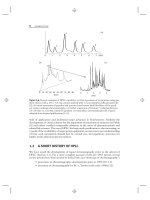
4.1 INTRODUCTION
The detector for the first liquid chromatographic separations was the human eye,
used by Tswett in his classic experiments [1, 2]. For many years quantitative
and qualitative analyses were accomplished by the collection of fractions eluted
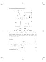
from the column (e.g., Fig. 4.1a), followed by off-line analysis using wet chemical,
gravimetric, optical, or other analysis techniques. The concentration of analyte in
each fraction could be plotted against fraction number, as in Figure 4.1b, resulting
in a crude chromatogram. Collection and analysis of fractions is time-consuming,
usually degrades chromatographic resolution, and is generally inconvenient, so
on-line detection has many benefits. Some of the first applications of on-line liquid
chromatographic detection included the refractive index detector reported by Tsielius
[3] and the conductivity detector by Martin and Randall [4]. However, it was the
introduction of the UV detector in 1966 by Horv
´
ath and Lipsky [5] that gave HPLC
its most widely used detector.
The UV detector was further improved in 1968 by Kirkland [6]; a flow-through
cell, plus use of a mercury lamp, resulted in a great improvement in sensitivity
(1 × 10
−5

AU noise). Single-wavelength detectors (254 nm) based on this principle
were by far the most popular through the 1970s—until they were subsequently
displaced by the variable-wavelength and diode-array UV detectors.
fraction number
off-line
analysis
(a)(b)
concentration
Figure 4.1 (a) Open-column LC; (b) plot of concentration of analyte in each fraction from (a).
4.2 DETECTOR CHARACTERISTICS 149
The chromatographic detector is a transducer that converts a physical or
chemical property of an eluted analyte into an electrical signal that can be related to
analyte concentration. Gas chromatography (GC) was well into its second decade
of popular use when HPLC began its rise to popularity. This gave GC a head
start in detector development as well. Much effort was given in the 1960s and
1970s to adapt GC detectors for HPLC use. A number of such detectors were
described, including flame ionization [7, 8], flame photometric [9], and electrolytic
conductivity [10]. However, adaptation of GC detectors required elimination of the
mobile phase through evaporation, and until the introduction of the electrospray
interface for LC-MS, the liquid-to-gas conversion process was very unreliable. As
a result GC-based detectors for HPLC were doomed by operational problems. It
was only after the development of an efficient nebulizer that detectors relying on
mobile-phase-elimination (LC-MS, evaporative light scattering, corona discharge,
FTIR, etc.) became practical.
Despite the lack of a universal, sensitive detector, such as the GC flame
ionization detector, there are many HPLC detectors that have been successful for
general or specific applications. This chapter describes the principles of operation
of the most popular HPLC detectors, presents example applications, and—where
appropriate—compares the advantages and disadvantages of specific detectors.
4.2 DETECTOR CHARACTERISTICS

The second edition of this book [11] listed nine characteristics of an ideal HPLC
detector:
• have high sensitivity and predictable response
• respond to all solutes, or else have predictable specificity
• be unaffected by changes in temperature and carrier flow
• respond independently of the mobile phase
• not contribute to extra-column peak broadening
• be reliable and convenient to use
• have a response that increases linearly with the amount of solute
• be nondestructive of the solute
• provide qualitative information on the detected peak
Of course, no detector possesses all of these characteristics, nor is likely to in
the foreseeable future. However, those HPLC detectors that have been the most
successful have many of the properties listed above.
4.2.1 General Layout
The HPLC detector is positioned directly after the column (Fig. 4.2) so as to minimize
post-column peak broadening (Section 3.9). The column effluent is directed into a
detector flow cell, where detection takes place. For most detectors the mobile phase
is maintained in a liquid state, detection occurs, and the mobile phase passes out
of the detector cell to a waste container, fraction collector, or another detector.
150 DETECTION
(a)(b)(c)
(d )(e)(f)
Figure 4.2 HPLC system diagram. (a) Mobile phase reservoir; (b) pump; (c) autosampler or
injector; (d) column; (e) detector; (f) data system.
The UV flow cell shown in Figure 4.3a has evolved into its present configuration,
in which the mobile phase flows through in a Z-shaped path, and UV light enters
the quartz window at one end of the cell. The differential absorbance of light is
monitored at the other end of the cell by a photosensitive diode, is converted to an
electrical signal, and eventually is presented by the data system as a chromatogram.

Different detectors have different flow-cell designs, as described in the following
detector-specific sections.
Optical detectors, such as UV and especially refractive index detectors, often
are sensitive to small temperature changes in the mobile phase, which cause changes
in the refractive index, and thus the amount of light that is transmitted through the
flow cell. To stabilize the temperature, the detector cell is mounted in a draft free,
and sometimes temperature-controlled, location in the detector case. The detector
commonly includes a capillary heat-exchanger to stabilize the incoming mobile-phase
temperature. One popular configuration is to wrap the capillary tubing around the
detector cell body and embed it in a thermally conductive sealant.
Detectors that make their measurements in the liquid state can be susceptible
to optical or electrical disturbances when bubbles are present. Thorough degassing
of the mobile phase (Section 3.3) often is sufficient to prevent bubble formation
within the detector. As an additional precaution a small back-pressure can be
applied to the detector outlet tube to prevent bubble formation. We recommend
that a spring-loaded check valve be purchased from an HPLC parts-supplier for this
purpose. If such a device is used, be careful that it does not exceed the pressure limit
of the cell. For example, use a back-pressure regulator that produces 50 to 75 psi of
back-pressure with a detector cell with a 150 psi pressure limit. Some workers rely
on the use of a piece of capillary tubing (e.g., 1 m × 0.005-in. i.d.) as a back-pressure
regulator. But the pressure created by such devices is proportional to the flow rate,
4.2 DETECTOR CHARACTERISTICS 151
light
out
end cap
quartz window
gasket
inlet
outlet
light

in
cell body
light
in
light
out
cell body
internal-
reflectance
coatin
g
(a)
(b)
Figure 4.3 UV-detector flow cells. (a) Typical construction of a Z-path flow cell; (b) light-pipe
flow cell lined with internally reflective surface.
so an increase in the pump flow rate can inadvertently create excessive back pressure
and cause cell leakage or damage.
4.2.2 Detection Techniques
There are four general techniques that are used for HPLC detection:
• bulk property or differential measurement
• sample specific
• mobile-phase modification
• hyphenated techniques
4.2.2.1 Bulk Property Detectors
A bulk property detector can be considered a universal detector as it measures a
property that is common to all compounds. The detector measures a change in
this property as a differential measurement between the mobile phase containing
the sample and that without the sample. The most familiar of the bulk property
detectors is the refractive index detector (Section 4.11). Bulk property detectors
have the advantage that they detect all compounds. The universal nature of bulk

mobile phase
152 DETECTION
property detectors can be a disadvantage, as well, because all components of the
sample that are eluted from the column will generate a detector signal. This means
that additional chromatographic selectivity may be needed to make up for the lack
of detection selectivity. As a general rule, universal detectors are inherently less
sensitive, since they rely on the difference between two large measurements (solvent
vs. solvent + solute).
4.2.2.2 Sample-Specific Detectors
Some characteristic of a sample is unique to that sample, or at least is not common
to all analytes, and the sample-specific detector responds to that characterstic.
The UV detector is the most commonly used sample-specific detector. It responds
to compounds that absorb UV light at a specific wavelength. The distinction
between bulk property detectors and sample-specific detectors is somewhat vague;
for example, at low wavelength (<210 nm), organic compounds all absorb in the UV
to some extent, so the UV detector becomes less selective and more universal at low
detection wavelengths. Other common sample-specific detectors rely on the ability of
an analyte to fluoresce (fluorescence, Section 4.5), conduct electricity (conductivity,
Section 4.8), or react under specific conditions (electrochemical, Section 4.6).
4.2.2.3 Mobile-Phase Modification Detectors
These detectors change the mobile phase after the column to produce a change in the
properties of the analyte. Such changes include a specific liquid-phase chemical reac-
tion with the analyte (reaction detectors, Section 4.16), a gas-phase reaction (e.g.,
corona discharge, Section 4.13; mass spectrometric detectors, Section 4.14), or cre-
ation of analyte particles suspended in a gas phase (e.g., evaporative light-scattering
detectors, Section 4.12.1).
4.2.2.4 Hyphenated Techniques
Hyphenated techniques refer to the coupling of an independent analytical instrument
to the HPLC system to provide detection, and often are abbreviated with a hyphen
as LC-(plus the technique). The most common hyphenated technique is LC-MS

(Section 4.14), where a mass spectrometer is coupled with an HPLC system. Other
less widely used techniques are LC-IR or LC-FTIR (Section 4.15.1) and LC-NMR
(Section 4.15.2). One can speculate at what point a detector is no longer considered a
hyphenated technique. Certainly the first UV detectors were UV spectrophotometers
fitted with flow-through cells, but now UV detectors are just another HPLC detector.
Generally, when the detector becomes widely used and the price of the detector is
in the same general range as the rest of the HPLC system, it can be considered a
detector. Thus it is reasonable to predict that mass spectrometers—which presently
cost 2- to 5-fold more than an HPLC system—will eventually be regarded as just
another HPLC detector.
4.2.3 Signal, Noise, Drift, and Assay Precision
The ability of a detector to provide precise and accurate quantitative data is a
function of the signal size generated by the analyte, background noise, and—to a
certain extent—baseline drift. Additional discussion of these topics is deferred to
Section 11.2.4.
4.2 DETECTOR CHARACTERISTICS 153
Response
drift
0 123456789101112
Time (min)
6
4
2
×10
4
AU
Time (min)
(a)
(b)
0102030405060708090

short-term
noise
Figure 4.4 Detector noise and drift. (a) Baseline, showing noise and drift; inset expanded to
show short-term noise; (b) long-term noise on baseline.
4.2.3.1 Noise and Drift
As defined in Figure 4.4, short-term noise is the baseline disturbance that occurs with
acycletimeof1 min (inset, Fig. 4.4a). Short-term noise is measured manually as
the peak-to-peak noise bracketing the extremes of the baseline (between dashed lines
of Fig. 4.4a; also shown in Fig. 4.7) in appropriate units (e.g., absorbance units for a
UV detector). Alternatively, short-term noise can be determined by the data-system
(usually with a root-mean-square calculation), if this feature is available. A common
contribution to short-term noise is the ‘‘buzz’’ on the baseline resulting from noise
contributed by motors or other appliances operated on the same electrical circuit
(as in Fig. 4.5). The frequency of this noise corresponds to the 60 Hz electrical
frequency, so it is referred to as 60-cycle noise (or 50-cycle in many countries).
Short-term noise often can be reduced or eliminated through the use of
electronic noise filtration. Most detectors have user-selectable noise filtration built
into their electronics. Alternatively, a resistance-capacitance (RC) filter can be built
using inexpensive components purchased from Radio Shack plus directions from
an introductory physics book. An example of the effectiveness of electronic noise
filtration is shown in Figure 4.5, where the noise on the raw signal is reduced by
≈300-fold through the application of an RC filter with a 1-sec time constant [12].
If the time constant is too large, it will also reduce the signal. As a rule of thumb,
if the time constant is less than ≈10% of the peak width, the peak signal will
not be compromised. For example, a 10,000 plate peak at k = 2 generated by a
154 DETECTION
0
Time
(
min

)
Response (mAU)
0
5
20
25
30
105
10
15
raw
signal
with 1-sec
time constant
Figure 4.5 Effect of a resistance-capacitance noise filter on detector noise. Raw detector signal
with ≈16 mAU short-term noise; 1-sec time constant reduces noise to <1mAU.
012345
Time (min)
0
−5
−10
−15
5
10
15
0
−5
−10
−15
5

10
15
Detector signal (μV)
(a)
(b)
Figure 4.6 Effect of data rate on detector noise. Baseline plots of data generated with (a)data
collection rate of 15 Hz and (b) 1 Hz (with data system input leads shorted). Adapted from
[12].
150 × 4.6-mm, 5-μm column operated at 1.5 mL/min would have a peak width of
≈7 sec, which would translate into a suitable time constant of ≤0.7 sec.
The data-system sampling rate (Section 11.2.1.1) also can affect short-term
noise. This is illustrated in Figure 4.6, where data sampling rates of 15 Hz (points per
4.2 DETECTOR CHARACTERISTICS 155
sec) and 1 Hz are compared [12]. The noise should be reduced by the square root of
the data rate change; therefore the change in the sampling rate from 15 Hz (Fig. 4.6a)
to 1 Hz (b) should reduce the noise ≈4-fold, as seen in Figure 4.6. The noise in
Figure 4.6 is reduced from ≈12 to ≈3 μV, although it looks like much more because
the high-frequency noise of Figure 4.6a is mostly eliminated in Figure 4.6b.Aruleof
thumb for setting the data sampling rate is to select a rate that collects ≥ 20 points
across a peak. For the N = 10,000, k = 2 example above (peak width ≈7 sec), a data
rate <7/20 sec or ≥ 20/7 sec
−1
≈ 3 Hz would be suitable. Remember that it is better
to err on the side of oversampling when the data are initially recorded; the data rate
can be reduced by post–run processing, but never increased (Section 11.2.1.1).
Although the detector time-constant (noise filtration) and the data-system
sampling rate (or data collection rate for processed data) both can be used to reduce
baseline noise, they accomplish this in a different manner. It is therefore wise to
evaluate both techniques (individually or in combination) to determine whether one
or a combination is more effective at noise reduction.

Long-term noise is the fluctuation in the baseline that occurs with a periodicity
in the same range as chromatographic peaks, as in Figure 4.4b. The longer period
of this type of noise means that electronic noise filtration will not be effective.
Long-term noise often is the result of elution of strongly retained materials from
previous runs. As retention is increased, peak width is increased, eventually to the
point where the peak deteriorates into baseline wander. A column flush with strong
solvent (e.g., 100% ACN or MeOH) will often reduce long-term noise.
Baseline drift is the gradual shift in the baseline over the course of one or more
runs, as illustrated by the heavy dashed line in Figure 4.4a. Baseline drift is common
with gradient elution because of the difference in detector response (the concentration
range over which the detector output is proportional to analyte concentration e.g.,
UV absorbance) between the starting and ending mobile phase (Section 17.4.5.1).
Baseline drift with UV detection can often be compensated by adding a nonretained,
UV-absorbing compound to the less-absorbant mobile-phase component (p. 178
of [13]). A change in the temperature of the mobile phase also can cause baseline
drift, especially for refractive-index detectors and other detectors that are sensitive
to refractive-index changes. Careful temperature control of the column, connecting
lines, and detector, as well as isolation of the entire HPLC system from drafts can
minimize drift. As long as the data system is able to adequately integrate peaks, a
moderately drifting baseline will not have any detrimental effect on data quality.
Short-term and long-term noise are superimposed on baseline drift, as seen in
Figure 4.4a. A good approach to minimize noise and drift problems is to (1) use
appropriate detector time-constants and data-system sampling rates, (2) regularly
flush the column with strong solvent, and (3) minimize temperature fluctuations
within and near the HPLC system. Remember that some baseline drift is common
in gradient elution, because of the difference in detector response to the A- and
B-solvents, and may not be changed by the practices above.
4.2.3.2 Signal-to-Noise Ratio (S/N)
This ratio is more important than either the signal or noise alone as an indicator
of detector performance for a particular peak. Noise is measured as described in

Section 4.3.2.1 for short-term noise, as shown in Figure 4.7. The signal is measured