Introduction to Modern Liquid Chromatography, Third Edition part 21 pdf

156 DETECTION
N
S
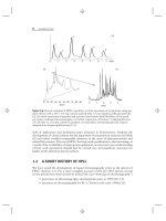
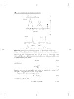
Figure 4.7 Measurement of chromatographic signal (S) and noise (N).
from the middle of the baseline noise to the top of the peak (Fig. 4.7). The
contribution of S/N to precision can be estimated as
CV =
50
S/N
(4.1)
where CV is the coefficient of variation (equivalent to %-relative standard deviation,
%-RSD). The lower limit of detection (LLOD) often is described as S/N = 3,
which would give CV ≈16%, whereas the lower limit of quantification (LLOQ)
is S/N = 10, for CV ≈5% (see also Section 11.2.4). These values of CV are
the contribution of S/N to the overall imprecision of the method, so the overall
method precision is expected to be worse than the S/N contribution. As long as the
imprecision attributable to S/N (or any other single contributor to error) is less than
half of the desired method imprecision, S/N will have a minor (<15%) influence on
the overall method precision (see the discussion of Eq. 11.2). For example, if the
overall method requires imprecision of no more than 2%, a contribution of S/N of
<1% should be satisfactory. This suggests that a S/N value of ratio 50:1 or more is
required for an overall method imprecision of <2%.
The signal-to-noise ratio can be improved by increasing the signal, reducing
the noise, or both, as summarized in Table 4.1. An increase in signal for a given
peak or sample may be available from a change in detector setting; for example, the
use of a UV wavelength that corresponds to maximum sample absorptivity. A more
sensitive detector also may be available, of either the same or different type.
Derivatization (Section 16.12) or other modification of the analyte may make
it more responsive to the chosen detector. A more common means of increasing
the signal is to inject a larger weight of sample (either a larger sample volume or
a sample concentrate; Section 3.6.3). However, column or detector overload will

eventually limit the possible increase in signal in this way. Any reduction in peak
width should translate into a proportional increase in peak height (area is assumed
to be constant); smaller k-values (increase in %B; see examples of Fig. 2.10b),
narrow-diameter columns, or more efficient small-particle columns can each be used
for this purpose.
4.2 DETECTOR CHARACTERISTICS 157
Table
4.1
Improvement of Signal-to-Noise Ratio
Increase Signal Decrease Noise
Better wavelength (or other detector adjustment) Increase detector time constant
More sensitive detector More data-system signal averaging
Analyte derivatization Better temperature control
Inject larger weight of sample Higher reagent/solvent purity
Reduce peak width (volumetric) Better sample cleanup
Smaller k Constant, pulse-free flow
Smaller column volume Column switching
Larger plate number
Any reduction of baseline noise also can improve S/N, for example, signal
smoothing by an increase in the detector time-constant or data-system sam-
pling rate (Section 4.2.3.1). Excessive smoothing, however, can reduce the signal
intensity. Better temperature control of the column, detector, and general instru-
ment environment also can reduce noise, especially for detectors sensitive to
refractive index changes. Purer solvents (e.g., HPLC grade) and better sam-
ple cleanup can reduce the introduction of noise-generating contaminants. For
gradient applications, changes in the system are sometimes attempted in order
to reduce the dwell-volume (Section 9.2.2.4) and the gradient delay time. The
mixer-volume comprises a major fraction of the dwell-volume in many systems,
but reduction of the mixer-volume can increase baseline noise. Some HPLC sys-
tems have optional mixers that can be added to smooth the baseline and reduce

noise—these devices can be especially advantageous for isocratic methods run
at maximum detector sensitivity. Column switching (Section 16.9) can be used
to transfer a desired fraction from a cleanup column to the analytical column,
thereby diverting unwanted contaminants to waste, so as to reduce baseline
noise.
4.2.4 Detection Limits
Although the signal-to-noise ratio is a measure of the inherent quality of the detector
signal, the minimum detectable mass or concentration often is the limiting factor
in the usefulness of a detector for a particular application. The term sensitivity
often is used interchangeably with detection limit when describing an HPLC detec-
tor. However, in proper use, sensitivity is the slope of a calibration plot, that
is, the change in signal per unit change in concentration (or mass) of analyte,
whereas detection limit refers to the minimum concentration (or mass) that can
be measured. HPLC detectors respond either to the concentration of the sample in
the detector cell (e.g., UV detection) or the mass of sample in the detector (e.g.,
LC-MS).
Detection limits, discussed more thoroughly in Section 11.2.5, are defined as
follows: The limit of detection LOD is the smallest signal that can be discerned
158 DETECTION
from the noise—with confidence that a peak really is present. Often a S/N of 3 is
equated to the LOD.Thelower limit of quantification LLOQ (sometimes called
limit of quantification or limit of quantitation, LOQ) is the smallest signal that can
be measured with the required precision for the method. The LLOQ often is defined
as S/N ≥ 10, but a value of S/N ≥ 50 may be chosen for high-precision methods.
There is a never-ending need for lower and lower detection limits for trace analysis,
and assays for which on-column injections of <1 ng are becoming more and more
common.
The LOD and LLOQ are directly related to the concentration (or mass) of
sample in the detector cell. Thus a longer path-length cell for UV detection is favored
in terms of signal intensity. However, the detector cell should be designed with

a minimum volume that is compatible with other requirements of the detector.
Excess cell volume will result in additional extra-column peak broadening (Section
3.9). This is especially true for small-volume columns, columns packed with small
particles, and peaks with k<2. For example, with a 50 × 4.6-mm column packed
with 3-μm particles and k<3, significant peak broadening was observed for an 8-μL
UV-detector cell when compared with a 1-μL cell [14]. To minimize the broadening
of early-eluted peaks, the detector cell volume V
det
should be less than approximately
one-tenth of the final volume of the peak of interest V
p
(V
p
= WF,whereW is the
baseline width of the peak [min], and F is flow rate [mL/min]) [15]:
V
det
< 0.1V
p
(4.2)
(For other peak-broadening contributions to V
p
, see Eq. 3.1 in Section 3.9.)
Some examples of the column contribution to peak volume V
p0
for early-eluted
peaks (k = 2) for some popular column configurations are shown in Table 4.2.
(In a well-behaved system, according to Eq. 2.27 and 3.1, the observed peak
volume V
p

should not be much larger than V
p0
.) Table 4.3 lists the detector cell
volumes for several UV-detector configurations. For UV detectors (Section 4.4),
signal intensity is proportional to path length, so longer path flow cells will have
lower detection limits. However, for detector cell diameters <1 mm, signal loss due
to light scattering in the cell can be a problem, so special cell designs (e.g., total
internal reflectance) are necessary for smaller cell diameters (see the discussion of
Section 4.4). The data of Tables 4.2 and 4.3 show that column lengths L ≥ 100
mm with a diameter d
c
= 4.6 mm, packed with 5- or 3-μm d
p
particles, will work
well with the standard 10 × 1.0-mm UV cell (see (Eq. 4.2), but any combination of
smaller column dimensions or smaller particles requires smaller cell volumes to avoid
unnecessary extra-column peak broadening. (Note that Eq. 3.1 is an approximation,
so peak-broadening calculations based on Eq. 3.1, and therefore conclusions based
on Tables 4.2 and 4.3, also are approximations.)
4.2.5 Linearity
For quantitative analysis by HPLC (Section 11.4), the detector response must
be related to the amount of analyte present. If analyte response y is plotted
against analyte concentration x, the simplest, most convenient, and most reliable
relationship is y = mx, where the slope m is a constant defined as the sensitivity.
Such a relationship between analyte response and analyte amount is termed linear.
4.2 DETECTOR CHARACTERISTICS 159
Table
4.2
Typical Peak Volumes V
p0

L (mm) d
c
(mm) d
p
(μm) V
p0
(μL)
a
250 4.6 5 212
150 4.6 5 164
3 127
2.1 3 26
100 4.6 3 104
2.1 3 22
1.0 3 5
24
50 4.6 3 73
2.1 3 15
2.1 2 12
1.0 2 3
a
Assumes k = 2; reduced plate height h = 2.5(seeEqs.2.27and3.1).
Table 4.3
UV-Detector Cell Volumes
Path Length (mm) Inner Diameter (mm) Volume (μL)
10 1.0 8
0.5 2
0.25 0.5
514
0.5 1

110.8
0.5 0.2
For best use over a wide range of sample concentrations, a wide linear dynamic range
(the concentration range over which the detector output is proportional to analyte
concentration, e.g., 10
5
for UV detection) is desired, so that both major and trace
components can be determined in a single analysis over a wide concentration range.
For example, with a stability-indicating method, peaks ≥ 0.1% of the response of
theactiveingredient(= 100%) must be reported, which would require a linear range
of at least 100/0.1 = 10
3
. Some detectors (e.g., evaporative light scattering) have a
narrow linear range of 1 to 2 orders of magnitude. Although less convenient and
reliable, a nonlinear calibration curve (e.g., quadratic) can be used—as long as the
detector response changes in a predictable manner with sample concentration (or
mass).
160 DETECTION
Table 4.4
HPLC Detectors
Sample-Specific
(Sections 4.4–4.10)
Bulk Property
(Sections 4.11–4.13)
Hyphenated
(Sections 4.14–4.15)
Reaction
(Section 4.16)
UV-visible Refractive index Mass spectrometric Reaction
Fluorescence Light scattering Infrared

Electrochemical Corona discharge Nuclear magnetic
resonance
Radioactivity
Conductivity
Chemiluminescent
nitrogen
Chiral
4.3 INTRODUCTION TO INDIVIDUAL DETECTORS
The remainder of this chapter (Sections 4.4–4.16) provides a discussion of most
HPLC detectors in use today. In Table 4.4, detectors are grouped by technique
(sample specific, bulk property, etc.) in approximate order of popularity within
each group. Sample-specific detectors will be treated first, and reaction detectors
last—with only limited discussion of less-used detectors. Within each section,
principles of detector operation are discussed first, followed by one or more
example applications. Where appropriate, a comparison with other detectors is
included.
A detailed discussion of every detector is beyond the scope of this book. In
addition to the references cited in each section, a more general discussion of HPLC
detectors can be found in [16, 17].
4.4 UV-VISIBLE DETECTORS
The most widely used detectors in modern HPLC are photometers based on ultravio-
let (UV) and visible light absorption. These detectors have a high sensitivity for many
solutes, but samples must absorb in the UV (or visible) region (e.g., 190–600 nm).
Sample concentration in the flow cell is related to the fraction of light transmitted
through the cell by Beer’s law:
log

I
o
I


= εbc (4.3)
where I
o
is the incident light intensity, I is the intensity of the transmitted light, ε is
the molar absorptivity (or molar extinction coefficient) of the sample, b is the cell
path-lengthincm,andc is the sample concentration in moles/L. Light-absorption
4.4 UV-VISIBLE DETECTORS 161
HPLC detectors usually are designed to provide an output in absorbance that is
linearly proportional to sample concentration in the flow cell,
A = log

I
o
I

= εbc (4.4)
where A is the absorbance.
Properly designed UV detectors are relatively insensitive to flow and temper-
ature changes. UV photometers that are linear to
>
2 absorbance units full scale
(AUFS) with <1 × 10
−5
AU noise are commercially available. With this perfor-
mance, solutes with relatively low absorptivities can be monitored by UV, and it is
possible to detect a few nanograms of a solute having only moderate UV absorbance.
The wide linear range of UV detectors (≈10
5
) makes it possible to measure both

trace and major components in the same chromatogram.
UV detectors commonly use flow cells of the Z-path design of Figure 4.3a,
with a 1-mm diameter and 10-mm path length (for a volume of ≈8 μL). This cell
volume is adequate for ≥100 ×≥4.6-mm columns packed with ≥3-μm particles
(Section 4.2.4), but smaller volume and/or smaller particle columns may experience
unacceptable extra-column peak broadening in an 8-μL cell. Shorter path-length
cells will reduce the cell volume, but the signal is proportional to the path length
(Eq. 4.4)—so sensitivity must be balanced against extra-column peak broadening in
choosing the flow cell dimensions. If the refractive index (RI) within the cell changes
(e.g., during gradient elution), the amount of energy reaching the photodetector can
change; when a light ray hits the side of the flow cell, the ratio of reflected to absorbed
light depends on the refractive-index ratio of the mobile phase and cell wall (and
the angle of the light ray hitting the cell wall). The latter refractive-index effect plus
imperfections in optical alignment make it difficult to successfully use cell diameters
smaller than ≈1 mm. One innovation that can minimize this problem is a flow cell
design as in Figure 4.3b, where the internal surface of the flow cell is coated with a
reflective coating—light that strikes the sides of the flow cell is reflected so as to still
reach the photodetector [18, 19]. The use of this light-pipe technique allows the cell
diameter to be reduced for smaller cell volumes (e.g., 0.25 mm × 10 mm ≈0.5 μL),
and thus less peak spreading for use with very small-volume, small-particle columns.
Alternatively, a longer, narrower diameter flow cell can be used (increasing b in Eqs.
4.3 and 4.4) for more absorbance in a smaller volume cell (e.g., 0.25 mm i.d. × 50
mm long, with a volume of ≈2.5 μL).
It is not necessary to operate a UV detector at the absorption maximum of the
analyte. A hypothetical example of wavelength selection is shown in Figure 4.8. The
spectra for two analytes, X and Y, are shown in Figure 4.8a, with UV maxima at
≈250 nm and ≈270 nm, respectively. At 280 nm, Y has much stronger absorbance,
so it has a much larger peak (Fig. 4.8b, same mass on column). At 260 nm, the
absorbances of X and Y are approximately equal, so the peaks are of approximately
equal size (Fig. 4.8c). At 210 nm, both compounds have even stronger absorbance

and generate much larger peaks (Fig. 4.8d). Notice also the appearance of a new
peak Z, which was not observed at higher wavelengths. This general increase in
sensitivity at lower wavelengths is one reason for the widespread use of ≤
220 nm for
detection
(near-universal detection). The corresponding loss of detector selectivity
at lower wavelengths can be a disadvantage for other separations, where it might
162 DETECTION
012345
Time (min)
280 nm
260 nm
210 nm
XY
X
Y
X
Y
Z
210 220 230 240 250 260 270 280
Wavelength (nm)
Absorbance
(a)
(b)
(c)
(d )
X
Y
Figure 4.8 Wavelength selectivity for UV detection. (a) Absorbance spectra for two hypo-
thetical compounds X and Y. Chromatograms at (b) 280 nm, (c) 260 nm, and (d) 210 nm.

be undesirable to ‘‘see’’ certain sample constituents (e.g., arising from the sample
matrix).
UV-visible spectrophotometric detectors can respond throughout a wide wave-
length range (e.g., 190–600 nm), which enables the detection of a broad spectrum
of compound types. Almost all aromatic compounds absorb strongly below 260 nm;
4.4 UV-VISIBLE DETECTORS 163
lamp filter beam
splitter
sample &
reference
flow cells
photocells
Figure 4.9 Schematic of a fixed-wavelength UV detector. Dashed lines show optical path.
compounds with one or more double bonds (e.g., carbonyls, olefins) can be detected
at wavelengths of <215 nm, while the preponderance of aliphatic compounds
possess significant absorbance at ≤205 nm. Reversed-phase mobile phases of ace-
tonitrile plus water or phosphate buffer can be used routinely for detection at
200 nm, whereas methanol-containing mobile phases cannot be used below ≈210
to 220 nm, depending on methanol concentration (see Appendix I, Table I.2). The
proper selection of the mobile phase makes it possible to operate UV detectors in
a near-universal detection mode in the 200- to 215-nm region, where most organic
compounds exhibit some UV absorbance. Because of the relatively small absorbance
differential between water (or phosphate buffer) and acetonitrile at
>
200 nm or
methanol at
>
220 nm, UV detectors are also quite useful for gradient elution.
Mobile phases with large differences in UV absorbance, such as tetrahydrofuran and
water at <240 nm, may not be amenable for use with gradients and UV detection.

UV detectors come in three common configurations. Fixed-wavelength detec-
tors (Section 4.4.1) rely on distinct wavelengths of light generated from the lamp,
whereas variable-wavelength (Section 4.4.2) and diode-array (Section 4.4.3) detec-
tors select one or more wavelengths generated from a broad-spectrum lamp.
4.4.1 Fixed-Wavelength Detectors
Figure 4.9 is a generic schematic of a fixed-wavelength UV detector. These detectors
were the mainstay of UV detection prior to the introduction of the variable- and
diode-array detectors, but they are not widely used today. Their current appeal is low
price and simple construction, and they tend to be more popular in the educational
environment or other budget-limited settings.
UV radiation at 254 nm from a low-pressure mercury lamp passes through a
band-pass filter and beam splitter, and shines on the entrance of the flow cell. Light
transmitted through the flow cell strikes the photodetector (usually a photodiode)
and is converted to an electronic signal. Most UV detectors operate in a differential
absorbance mode, where light also passes through a reference cell, and the difference
between the light passing through the sample and reference cells is converted
to absorbance, according to Equation (4.4). Although some detectors enable the
reference cell to be filled with mobile phase, an air reference is most commonly used,
which allows for correction of variations in light intensity from the source lamp, but
not for changes in the mobile-phase absorbance.
164 DETECTION
lamp
diffraction
grating
slit
flow cell
photocell
200 nm
360 nm
Figure 4.10 Schematic of a variable-wavelength UV detector; reference flow cell not shown.

Dashed lines show optical path.
The 254-nm line from the low-pressure mercury lamp is the most popular
wavelength for use with the fixed-wavelength UV detector. For historical reasons
this wavelength is still popular for applications that use variable- and diode-array
detectors, although there is no real reason to use this particular wavelength. Through
the use of other lamps (e.g., zinc), phosphors, and other lines in the mercury lamp
output, detection at 214, 220, 280, 313, 334, and 365 nm can be accomplished with
the fixed-wavelength detector.
4.4.2 Variable-Wavelength Detectors
UV spectrophotometers (variable-wavelength and diode-array detectors) offer a
wide selection of UV and visible wavelengths. Such devices have the versatility and
convenience of operation at the absorbance maximum of a solute or at a wavelength
that provides maximum selectivity, as well as the ability to change wavelengths
during a chromatographic run.
The most widely used detector in HPLC today is the variable-wavelength UV
detector shown schematically in Figure 4.10. A broad-spectrum UV lamp (typically
deuterium) is directed through a slit and onto a diffraction grating. The grating
spreads the light out into its component wavelengths, and the grating is then rotated
to direct a single wavelength (or narrow range of wavelengths) of light through the
slit and detector cell and onto a photodetector. These detectors usually use a sample
and reference cell configuration (Section 4.4) for differential detection. For detection
in the visible region, a tungsten lamp is used instead of deuterium.
The use of a variable-wavelength detector allows one to program a change in
the detection wavelength during a chromatogram. Thus one peak can be detected at
280 nm and another at 220 nm. Although it is possible for many detector models
to change the wavelength quickly, so as to generate a UV spectrum for a peak, the
results are complicated by the change in analyte concentration during the spectral
scan and may be of limited value.
4.4 UV-VISIBLE DETECTORS 165
lam

p
slit
flow cell
photodiode
array
diffraction
grating
200 nm
360 nm
Figure 4.11 Schematic of a diode-array UV detector. Dashed lines show optical path.
4.4.3 Diode-Array Detectors
A schematic of the diode-array detector (DAD, also called photodiode-array, PDA)
is shown in Figure 4.11; it has a similar optical path to the variable-wavelength
detector, except that the white light from the lamp passes through the flow cell prior
to striking the diffraction grating. This allows the grating to spread the spectrum
across an array of photodiodes, hence the name photodiode array (PDA). The number
of photodiodes varies with the specific brand and model of detector, but detectors
with 512 or 1024 diodes are common. The signals from the individual photodiodes
are processed to generate a spectrum of the analyte. Because the spectra are generated
at the same time (vs. single-wavelength monitoring with the variable-wavelength
detector), the DAD can contribute to peak identification. The DAD can be operated
to collect data at one or more wavelengths across a chromatogram, or to collect full
spectra on one or more analytes in a run. Of course, the data-file size is much larger
for full-spectra runs, but data compression techniques and inexpensive data storage
make this less of a concern than it was in the past.
If two closely eluted peaks have sufficiently different spectra, it may be possible
to distinguish the two peaks spectrally. The utility of the DAD to distinguish
between two peaks can be understood in conjunction with Figure 4.12, where a
partial chromatogram for a closely eluted peak pair X and Y is shown (Fig. 4.12a).
If the solutes have spectra as shown in Figure 4.12b and are monitored at a

wavelength where both have significant absorbance, such as 260 nm, the resulting
chromatogram will look like a single peak (X + Y in Fig. 4.12a); the corresponding
peaks are shown for the solutes injected individually. Even though the peaks appear
to overlap completely at 260 nm, if other wavelengths are monitored, it may be
possible to distinguish between the peaks. For example, if 240 nm is used, only X
will respond, whereas only Y will respond at 280 nm. The added selectivity of the
detector can be used to compensate, at least in part, for inadequate chromatographic
separation. Thus the DAD could simultaneously collect data at 240 and 280 nm
during the chromatographic run, and individual chromatograms plotted at 240 or
280 nm would allow quantification of X and Y, even under the partially overlapped
conditions of Figure 4.12.
Another common application of the DAD is for peak-purity determination. The
software accompanying the DAD accomplishes this by calculating an absorbance