Introduction to Modern Liquid Chromatography, Third Edition part 46 pptx

406 GRADIENT ELUTION
9.1.1 Other Reasons for the Use of Gradient Elution
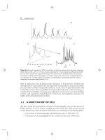
Apart from the need for gradient elution in the case of wide-polarity-range samples
like that of Figure 9.1, there are a number of other situations that favor or require
the use of gradient elution:
• high-molecular-weight samples
• generic separations
• efficient HPLC method development
• sample preparation
• peak tailing
High-molecular-weight compounds, such as peptides, proteins, and oligonu-
cleotides, are usually poor candidates for isocratic separation, because their retention
can be extremely sensitive to small changes in mobile-phase composition (%B). For
example, the retention factor k of a 50,000-Da protein can change by 3-fold as a
result of a change in the mobile phase by only 1% B. This behavior can make it
extremely difficult to obtain reproducible isocratic separations of macromolecules in
different laboratories, or even within the same laboratory. Furthermore the isocratic
separation of a mixture of macromolecules usually results in the immediate elution
of some sample components (with k ≈ 0 and no separation), and such slow elution
of other components (with k  100) that it appears that the sample never leaves the
column; that is, the retention range of such samples is often extremely wide (isocratic
k-values for different sample components that vary by several orders of magnitude).
With gradient elution, on the other hand, irreproducible retention times for large
molecules are seldom a problem, and resulting separations can be fast, effective, and
convenient (Chapter 13).
Generic separations are used for a series of samples, each of which is made
up of different components; for example, compounds A, B,andC in sample 1,
compounds D, E,andF in sample 2, and so forth. Typically each sample will
be separated just once within a fixed separation time (run time), with no further
method development for each new sample. In this way hundreds or thousands of
related samples—each with a unique composition—can be processed in minimum

time and with minimum cost. Generic separations by RPC (with fixed run times,
for automated analysis) are only practical by means of gradient elution and are
commonly used to assay combinatorial libraries [3], as well as other samples [4].
Generic separation is often combined with mass spectrometric detection [5], which
allows both the separation and identification of the components of samples of
previously unknown composition—without requiring the baseline resolution of
peaks of interest.
Efficient HPLC method development [6] is best begun with one or more
gradient experiments (Section 9.3.1). A single gradient run at the start of method
development can replace several trial-and-error isocratic runs as a means for estab-
lishing the best solvent strength (value of %B) for isocratic separation. An initial
gradient run can also establish whether isocratic or gradient elution is the best choice
for a given sample.
Sample preparation (Chapter 16) is required in many cases because some
samples are unsuitable for direct injection followed by isocratic elution. Interfering
9.1 INTRODUCTION 407
peaks, strongly retained components, and particulates must first be removed. In some
cases, however, gradient elution can minimize (or even eliminate) the need for sample
preparation. For example, by spreading out peaks near the beginning of a gradient
chromatogram (as in Fig. 9.1g vs.Fig.9.1a), interfering peaks (non-analytes) that
commonly elute near t
0
can be separated from peaks of interest. Similarly strongly
retained non-analytes at the end of an isocratic separation can result in excessive
run times, because these peaks must clear the column before injection of the next
sample. Gradient elution can usually remove these late-eluting compounds within a
reasonable run time (Section 9.2.2.5).
Peak tailing was a common problem in the early days of chromatography, and
the reduction of tailing was an early goal of gradient elution [7]. Because of the
increase in mobile-phase strength during the time a band moves through the column

in gradient elution, the tail of the band moves faster than the peak front, with
a resulting reduction in peak tailing and peak width (Section 9.2.4.3). However,
peak tailing is today much less common, and other means are a better choice for
addressing this problem when it occurs (Section 17.4.5.3).
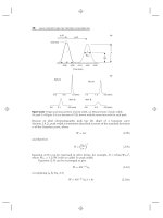
9.1.2 Gradient Shape
By gradient shape, we mean the way in which mobile-phase composition (%B)
changes with time during a gradient run. Gradient elution can be carried out with
different gradient shapes, as illustrated in Figure 9.2a–f. Most gradient separations
use linear gradients (Fig. 9.2a), which are strongly recommended during the initial
stages of method development. Curved gradients (Fig. 9.2b,c) have been used in the
past for certain kinds of samples, but for various reasons such gradients have been
largely replaced by segmented gradients (Fig. 9.2d). Segmented gradients can provide
most of the advantages of curved gradients, are easier to design for different samples,
and can be replicated by most gradient systems. The use of segmented gradients
for various purposes is examined in Section 9.2.2.5. Gradient delay or ‘‘isocratic
hold’’ (Section 9.2.2.3) is illustrated by Figure 9.2e; an isocratic hold can also be
used at the end of the gradient. Step gradients (Fig. 9.2f), where an instantaneous
change in %B is made during the separation, are a special kind of segmented
gradient. They are used infrequently—except at the end of a gradient separation for
cleaning late-eluting compounds from the column; a sudden increase in %B (as in i
of Fig. 9.2f) achieves this purpose. A step gradient that provides a sudden decrease
in %B (as in ii of Fig. 9.2f) can return the gradient to its starting value for the next
separation. In the past, step gradients were sometimes avoided because of a concern
for column stability; with today’s well-packed silica-base columns, however, step
gradients can be used without worry about column damage.
A linear gradient can be described (Fig. 9.2g) by the initial and final
mobile-phase compositions, and gradient time t
G
(the time from start-to-finish
for the gradient). We can define the initial and final mobile-phase compositions in

terms of %B, or we can use the volume-fraction φ of solvent B in the mobile phase
(equal to 0.01%B): values φ
o
and φ
f
, respectively. The change in %B or φ during
the gradient is defined as the gradient range andisdesignatedbyΔφ = φ
f
− φ
0
(or
the equivalent Δ%B = [final%B] − [initial%B]). In the present book, values of %B
and φ will be used interchangeably; that is, φ always equals 0.01%B, and 100% B
(φ = 1.00) signifies pure organic solvent in RPC. For reasons discussed in Section
408 GRADIENT ELUTION
%B
%B
%B
%B
%B
%B
time time
Concave Segmented
(a)
(c)
(e)
(g)
time time
Linear Convex
(b)

(d)
(f )
(h)
time
time
Gradient
delay
Step gradients
i
ii
100
80
60
40
20
0
100
80
60
40
20
0
0 5 10 15 2
0
(min)
5/25/40/100% B
at 0/5/15/20min
t
G
= 20 min

= (0.80 – 0.10) = 0.70
%B
0 5 10 15 20
(min)
10-80% B
in 20 min
o
= 10% B ≡ 0.10
f
= 80% B ≡ 0.80
=
f
–
o
Figure 9.2 Illustration of different gradient shapes (plots of %B vs. time).
17.2.5.3, it is sometimes desirable for the A- and/or B-solvent reservoirs to contain
mixtures of the A- and B-solvents, rather than pure water and organic, respectively;
for example, 5% acetonitrile/water in the A-reservoir and 95% acetonitrile/water in
the B-reservoir. For the latter example, a (nominal) 0–100% B gradient would then
correspond to 5–95% acetonitrile, with Δφ = (0.95 – 0.05) = 0.90.
9.1 INTRODUCTION 409
By a gradient program, we refer to a description of how the mobile-phase
composition changes with time during a gradient. Linear gradients represent the
simplest program, for example, a gradient from 10–80% B in 20 minutes (Fig. 9.2g),
which can also be described as 10/80% B in 0/20 min (10% B at 0 min to 80% B at
20 min). Segmented programs are usually represented by values of %B and time for
each linear segment in the gradient, for example, 5/25/40/100%B at 0/5/15/20 min
for Figure 9.2h.
9.1.3 Similarity of Isocratic and Gradient Elution
A peak moves through the column during gradient elution in a series of small steps,

in each of which there is a small change in mobile-phase composition (%B). That
is, gradient separation can be regarded as the result of a large number of small,
isocratic steps. Separations by isocratic and gradient elution can be designed to
give similar results. The resolution achieved for selected peaks in either isocratic
or gradient elution will be about the same, when average values of k in gradient
elution (during migration of each peak through the column) are similar to values of
k in isocratic elution, and other conditions (column, temperature, A- and B-solvents,
etc.) are the same. Isocratic and gradient separations where the latter conditions
apply are referred to as corresponding. Thus the isocratic examples of Figure 9.1b–f
can be compared with the ‘‘corresponding’’ gradient separation of Figure 9.1g.The
isocratic separations of individual groups of peaks in Figure 9.1b–f each occur
with k ≈ 3, while in the gradient separation of Figure 9.1g the equivalent value of
k for each peak is also ≈ 3. We see in this example that the peak resolutions of
Figure 9.1b–f are similar to those of Figure 9.1g.
In isocratic elution we can change values of k by varying the mobile-phase
strength (%B). In gradient elution, average values of k can be varied by changing
other experimental conditions—as described below in Section 9.2.
9.1.3.1 The Linear-Solvent-Strength (LSS) Model
This section provides a quantitative basis for the treatment of gradient elution in this
chapter. However, the derivations presented here are of limited practical utility per
se (although necessary for a quantitative treatment of gradient elution). The reader
may wish to skip to Section 9.1.3.2 and return to this section as needed.
Isocratic retention in RPC is given as a function of %B (Section 2.5.1) by
log k = log k
w
− Sφ (9.1)
For a given solute, the quantity k
w
is the (extrapolated) value of k for φ = 0(water
or buffer as mobile phase), and S ≈ 4 for small molecules (<500 Da). A linear

gradient can be described by
%B = (%B)
0
+

t
t
G

[(%B)
f
− (%B)
0
] (9.2)
Here %B refers to the mobile-phase composition at the column inlet, (%B)
0
is the
value of %B at the start of the gradient (time zero), (%B)
f
is the value of %B at the
410 GRADIENT ELUTION
finish of the gradient, t is any time during the gradient, and t
G
is the gradient time.
We can restate Equation (9.2) in terms of φ, the volume-fraction of B:
φ = φ
0
+

t

t
G

(φ
f
− φ
0
)
= φ
0
+

Δφ
t
G

t (9.2a)
where φ
0
is the value of φ at the start of the gradient, φ
f
is the value of φ at the end of
the gradient, and Δφ = (φ
f
− φ
0
) is the change in φ during the gradient (the gradient
range); see Figure 9.2g. The quantity φ refers to values at the column inlet, measured
at different times t during the gradient. Thus the mobile-phase composition at time
t = 0 (the start of the gradient) is φ = φ

0
, provided that no delay occurs between the
gradient mixer and the column inlet (Section 9.2.2.3).
Equations (9.1) and (9.2a) can be combined to give
log k = log k
w
− Sφ
0
−

ΔφS
t
G

t
= C
1
− C
2
t (9.3)
For a linear gradient, a given solute, and specified experimental conditions C
1
and
C
2
are constants, so log k varies linearly with time t during the gradient (the value
of k in Eq. 9.3 refers to the value of k measured at the column inlet at any given
time t). Gradients for which Equation (9.3) applies are called linear-solvent-strength
(LSS) gradients; linear RPC gradients are therefore (approximately) LSS gradients.
Exact equations for retention and peak width can be derived for LSS gradients

(Section 9.2.4). LSS separations are much easier to understand and to control,
compared to the use of other gradient shapes. Finally, LSS gradients provide a better
separation of most samples that require gradient elution.
A fundamental definition of gradient steepness b for a given solute is
b =
V
m
ΔφS
t
G
F
(9.4)
or as t
0
= V
m
/F,
b =
t
0
ΔφS
t
G
(9.4a)
This definition of gradient steepness follows from Equation (9.3), which can be
written as
log k = log k
w
− Sφ
0

−

t
0
ΔφS
t
G

t
t
0

or
log k = log k
w
− Sφ
0
− b

t
t
0

(9.4b)
9.1 INTRODUCTION 411
where (log k
w
− Sφ
0
) for a given gradient and solute is equal to log k at the start

of the gradient (and therefore varies with φ
0
; see later Eq. 9.7). A larger value of
b corresponds to a faster decrease in k with time, or a steeper gradient. Retention
times and peak widths in gradient elution can be derived from the relationships
above (see Section 9.2.4).
9.1.3.2 Band Migration in Gradient Elution
Consider next how individual solute bands move through the column during gradient
elution (Fig. 9.3). For an initially eluted compound i in Figure 9.3a, the solid curve
(x[i]) marks the fractional migration x of band i through the column as a function
of time (note that y = 1onthey-axis represents elution of the band from the
column; y = 0 represents the band at the column inlet). Band migration is seen to
accelerate with time, resulting in an upward-curved plot of x versus t. Also plotted
in Figure 9.3a is the instantaneous value of k for band-i (dashed curve, k[i]) as it
migrates through the column. The quantity k(i) is the value of k at time t for an
isocratic mobile phase whose composition (%B) is the same as that of the mobile
phase in contact with the band at time t.Peakwidthandresolutioningradient
elution depend on the median value of k: the instantaneous value of k when the
k(i) k(j )
x(i) x(j)
1.0
0.0
5
3
1
k
Band migration x
k*
k
e

024681012141618
Time (min)
i j
5 10 15 (min)
(a)
(b)
Figure 9.3 Peak migration during gradient elution. (a) Band-migration x and instantaneous
values of k related to time, showing average (k
∗
) and final values of k (at elution, k
e
); (b)result-
ing chromatogram.
412 GRADIENT ELUTION
band has migrated halfway through the column. This median value of k in gradient
elution is defined as the gradient retention factor k
∗
. Peak width is determined by the
value of k when the peak leaves the column (defined as k
e
,equaltok
∗
/2). A similar
plot for a second band j (with values of x = x[j], and k = k[j]) is also shown in
Figure 9.3a. The resulting chromatogram for the separation of Figure 9.3a is shown
in Figure 9.3b.
A comparison of band migration in Figure 9.3a for the two compounds i and
j shows a generally similar behavior, apart from a delayed start in the migration of
band j because of its stronger initial retention (larger value of k
w

). Specifically, values
of k
∗
and k
e
for both early and late peaks in the chromatogram are approximately
the same for solutes i and j, suggesting that resolution and peak spacing need not
decrease for earlier peaks, as in isocratic elution for small values of k (compare
the gradient separation of peaks 1–6 in Fig. 9.1e with their isocratic separation in
Fig. 9.1a). Values of k
e
are also usually similar for early and late peaks in gradient
elution, meaning that peak widths (and heights) will be similar for both early and
late peaks in the chromatogram (contrast the peak heights for peaks 1–14 in the
gradient separation of Fig. 9.1e with these same peaks in the isocratic separation
of Fig. 9.1a). The relative constancy of values of k* and k
e
for a linear-gradient
separation are responsible for the pronounced advantages of gradient over isocratic
elution for the separation of wide-range samples such as that of Figure 9.1.
9.2 EXPERIMENTAL CONDITIONS AND THEIR EFFECTS
ON SEPARATION
The gradient retention factor k
∗
of Figure 9.3 has a similar significance in gradient
elution as the retention factor k has in isocratic elution. Values of k in isocratic
elution are important for the understanding and control of separation, and we will
see that values of k
∗
play the same role in gradient elution. The value of k

∗
depends
on the solute (its value of S in Eq. 9.1) and experimental conditions: gradient time
t
G
, flow rate F, column dimensions, and the gradient range Δφ [2]:
k
∗
=
0.87t
G
F
V
m
ΔφS
(9.5)
Here V
m
is the column dead-volume (mL), which can be determined from an
experimental value of t
0
and the flow rate F (Section 2.3.1; V
m
= t
0
F). Values of
S for different samples with molecular weights in the 100 to 500 Da range can be
assumed equal to about 4. This means that values of k* for different solutes in a
given linear-gradient separation (with constant values of t
G

, F, V
m
, and Δφ) will all
be about the same.
Let us next compare isocratic and gradient separation in terms of values of k
and k
∗
, for the same sample and similar conditions (same A- and B-solvents, column,
flow rate, and temperature). The isocratic separations of Figure 9.4a–c illustrate
the effect of a change in %B (and k), for mobile phases of 70, 55, and 40% B.
Similar values of k
∗
in gradient elution can be achieved by varying gradient time
t
G
(Eq. 9.5 with S = 4); see Figure 9.4d–f ,wherek
∗
= 1, 3, and 9 for t
G
= 3, 10,
9.2 EXPERIMENTAL CONDITIONS AND THEIR EFFECTS ON SEPARATION 413
and 30 minutes, respectively. Isocratic and gradient separations will be referred to
as ‘‘corresponding’’ when the average value of k in the isocratic separation equals
the value of k
∗
for the gradient separation (for the same sample and experimental
conditions, except that %B and k
∗
are allowed to vary). In the example of Figure 9.4,
separations (a)and(d) are ‘‘corresponding,’’ as are separations (b)and(e), and

(c)and(f ). ‘‘Corresponding’’ separations as in these examples should be similar in
terms of resolution and average peak heights—except that peaks in the gradient
separation can be taller by as much as 2-fold.
For either isocratic or gradient elution, an increase in k or k
∗
corresponds to
an increase in run time (other conditions the same). In isocratic elution, resolution
increases for larger values of k (Eq. 2.24), as observed in Figure 9.4a–c (R
s
= 0.4,
1.7, and 3.4). For similar values of k
∗
in gradient elution (Fig. 9.4d–f), the observed
resolution is seen to be about the same for each ‘‘corresponding’’ separation
(R
s
= 0.4, 1.7, and 3.6). Finally, peak widths in isocratic elution increase with k
(decrease in %B), resulting in decreased peak heights. Again, similar changes in peak
width and height are observed in gradient elution as k
∗
is varied in Figure 9.4d–f .
Thus changes in %B for isocratic elution, or gradient time in gradient elution, lead
to similar changes in run time, resolution, and peak heights.
0246
Time (min)
70% B
R
s
= 0.4
1

2
3
4
5
1
2
3
4
5
01020
Time (min)
(a)
(b)
(c)
02
Time (min)
1
+
2
3
4
5
t
0
1 ≤ k ≤ 2
55% B
R
s
= 1.7
2 ≤ k ≤ 8

40% B
R
s
= 3.4
6 ≤ k ≤ 23
Figure 9.4 Isocratic (a–c) and gradient (d–f) separations compared for a regular sample
and change in either %B or gradient time. Sample: 1, simazine, 2, monolinuron; 3, metobro-
muron; 4, diuron; 5, propazine. Conditions: 150 × 4.6-mm C
18
column (5-μm particles);
methanol-water mobile phase (%B or gradient conditions indicated in figure); ambient tem-
perature; 2.0 mL/min. Note that actual peak heights are shown (not normalized to 100% for
tallest peak). Chromatograms recreated from data of [8].
414 GRADIENT ELUTION
2.2 2.4 2.6 2.8 3.0 3.2 3.4
Time (min)
1
+
2
4
5
3
6.0 7.0 8.0
Time (min)
1
2
3
4
5
10 12 14 16 18

Time (min)
1
2
3
4
5
0-100% B in 3 min
k* = 1
R
s
= 0.4
0-100% B in 10 min
k* = 3
R
s
= 1.7
0-100% B in 30 min
k* = 9
R
s
= 3.6
(d)
(e)
(f )
Figure 9.4 (Continued)
The sample of Figure 9.4 can be described as ‘‘regular’’ (Section 2.5.2.1)
because there are no changes in relative retention when k or k
∗
are varied by varying
isocratic %B or gradient time, respectively (holding other conditions constant).

Consequently critical resolution increases continuously in Figure 9.4d–f as gradient
time (and k
∗
) is increased. A similar series of experiments are shown in Figure 9.5
for an ‘‘irregular’’ sample (Section 2.5.2.1), composed of a mixture of substituted
anilines and benzoic acids. Relative retention for an ‘‘irregular’’ sample changes as
either isocratic %B or gradient time is varied. As in Figure 9.4, the same trends in
average resolution, peak heights, and run time result in Figure 9.5 when gradient
time is increased. However, changes in relative retention also occur for the sample of
Figure 9.5 when gradient time is changed (note the changes in relative retention of
shaded peak 3 and—to a lesser extent—peaks 7–10). As a result of these changes
in relative retention with t
G
, maximum (‘‘critical’’) resolution for this sample occurs
for an intermediate gradient time of 10 minutes (Fig. 9.5b; R
s
= 0.9), whereas the
resolution of the ‘‘regular’’ sample in Figure 9.4 continues to increase as gradient
time (and k
∗
) increases. For ‘‘irregular’’ samples a change in either k (isocratic) or k
∗
(gradient) will result in similar changes in relative retention; consequently maximum
sample resolution may not correspond to the largest possible value of k or k
∗
for
such samples.
9.2 EXPERIMENTAL CONDITIONS AND THEIR EFFECTS ON SEPARATION 415
0
246

Time (min)
02
Time (min)
3-min gradient
k* = 1.5, R
s
= 0.4
10-min gradient
k* = 5, R
s
= 0.9
30-min gradient
k*= 15, R
s
= 0.1
(a)
(b)
(c)
1
4
5
+
6
1
2
3
4
5 − 7
9
8

10
11
2
7
+
8
9
11
10
024681012
Time
(
min
)
2
+
3
4
8
10
11
1
9
5 - 7
3
Figure 9.5 Separations of an irregular sample as a function of gradient time t
G
. Sample: a mix-
ture of substituted anilines and benzoic acids. Conditions: 100 × 4.6-mm C
18

column (3-μm
particles), 2.0 mL/min, 42
◦
C, 5–100% acetonitrile-pH-2.6 phosphate buffer in (a)5min-
utes, (b) 15 minutes, and (c) 30 minutes. Peak 3 is cross-hatched to better illustrate changes
in relative retention for this sample as gradient time is varied. Note that actual peak heights are
shown (not normalized to 100% for tallest peak). Chromatograms recreated from data of [9].
9.2.1 Effects of a Change in Column Conditions
Column conditions—column length and diameter, flow rate, and particle
size—affect the column plate number N (Section 2.4.1) and run time. Column
conditions are chosen at the start of method development, then sometimes changed
after other separation conditions have been selected—in order to either improve
resolution or reduce run time (Section 2.5.3). In isocratic elution, a change in
column conditions has no effect on values of k or relative retention. Resolution
and run time usually increase for an increase in column length or a decrease in
flow rate, while peak heights decrease for longer columns and faster flow. These
changes in isocratic separation, when only column length or flow rate is changed,
are illustrated in Figure 9.6a–c for the ‘‘regular’’ sample of Figure 9.4. Figure 9.6a
represents a starting separation, while Figures 9.6b and 9.6c show the results of
an increase in either column length or flow rate, respectively. Note the resulting