Introduction to Modern Liquid Chromatography, Third Edition part 79 pot

736 PREPARATIVE SEPARATIONS
phase is no longer a minor issue. The major difficulty is the elimination of water,
which has a higher boiling point and higher heat of vaporization than typical organic
solvents—resulting in long evaporation times. This not only limits the quantity of
material that can be isolated in a given time but also exposes the product to a
higher temperature during prolonged evaporation; this can lead to degradation of
the product. For these reasons many chromatographers routinely select nonaqueous
NPC (Section 8.4) for prep-LC. For NPC carried out with solvents that boil below
80
◦
C (see Table I.3 of Appendix I), the recovery of purified product is relatively
simple. NPC is also often favored by a potentially larger value of the separation
factor α, which corresponds to larger allowable sample weights (as in the example of
Figure 15.2; see also Section 15.3.2); this is especially true for closely related solutes
such as isomers (Section 8.3.5).
RPC is not ruled out for prep-LC separation, as there are several options
for the recovery of solvent-free product—depending on the nature of the product.
Additionally any required buffers or additives can be selected from a list of volatile
compounds (Section 7.2.1) to avoid the necessity of salt removal from the product.
Many compounds are relatively insoluble in water, especially at a pH where they are
not ionized: for example, a strongly acidic pH for an acid or an alkaline pH for a
base (see Tables 7.2, 13.1, and 13.8 for solute pK
a
values as a function of compound
molecular structure). The appropriate adjustment of the pH of a product fraction,
followed by partial evaporation of the fraction in order to eliminate most of the
organic solvent, will often precipitate most of the product and allow its recovery
by filtration. An alternative approach is the continuous extraction of the (partly
aqueous) fraction with a water-immiscible organic solvent. The product is thus
partitioned into an organic solvent which is then easily removed by evaporation.
Either of these approaches also leaves any (nonvolatile) inorganic buffer behind in

the aqueous phase.
In other cases dilution of the fraction with water, followed by passage through a
solid-phase extraction (SPE) cartridge (Section 16.6), may allow the desired product
to be retained by the cartridge. The cartridge can then be washed with water to
remove nonvolatile buffer or salt, following which the product can be eluted from
the cartridge with a water-miscible organic solvent that is more easily evaporated.
Any small amount of water remaining in the product-fraction after SPE can be
removed by azeotropic distillation in a rotary evaporator—following the addition
of a suitable solvent that can form a volatile azeotrope with water. Chloroform is
especially useful for this purpose, as any remaining water will be visually apparent
as immiscible droplets. Because only 3% of a chloroform/water distillate is water,
this process may need to be repeated once or twice to complete the removal of water.
Other solvents (e.g., ethanol, dichloromethane) can also be used. Reference to tables
of physical properties of solvent mixtures [3] can be helpful in finding a suitable
azeotroping solvent.
The removal of water by lyophilization may be preferred for less stable, very
water-soluble products. Prior elimination of nonvolatile buffers or additives may be
required initially, as by ion-exchange chromatography (Section 16.6.2.3). Because
the product is held at a temperature <0
◦
C, lyophilization is commonly used for
protein products, in order to prevent their denaturation or decomposition during
drying.
15.3 ISOCRATIC ELUTION 737
15.3 ISOCRATIC ELUTION
Since 1980 there have been dramatic advances in our understanding and use of
prep-LC. The group of Guiochon, in particular, has developed an extensive math-
ematical treatment of preparative chromatography, especially for large-scale, non-
touching peak separations [4]. For separations on the laboratory scale (Table 15.2),
the general principles of prep-LC are more useful than involved mathematical treat-

ments that require computer calculations for their implementation. The present
chapter will emphasize these general principles.
15.3.1 Sample-Weight and Separation
The present section provides a fundamental understanding of how column overload
affects separation, but it has limited immediate application. For this reason the
reader may prefer to skip to Section 15.3.2, and return to the present section as
appropriate.
15.3.1.1 Sorption Isotherms
The sorption isotherm describes the distribution of the solute between the stationary
and mobile phases at a given temperature, as a function of solute concentration
in the mobile phase. Most HPLC separations obey the Langmuir isotherm,which
describes the distribution of solute molecules between the mobile and stationary
phases:
C
s
=
aC
m
1 + b
∗
C
m
(15.1)
Here C
s
is the concentration of solute in the stationary phase, C
m
is the solute
concentration in the mobile phase, and a and b
∗

are constants for a given solute,
mobile phase, stationary phase, and temperature. This model of sample uptake by
the column assumes that solute retention takes place onto a planar surface with a
defined maximum capacity—the filled adsorbed monolayer (Sections 8.2.1, 15.3.2.1;
Fig. 15.6a).
For small solute concentrations C
m
, C
s
= aC
m
, and from Equation (15.1),
k =
C
s
V
s
C
m
V
m
=
C
s
/C
m
V
s
/V
m

= K (15.2)
where V
s
and V
m
are, respectively, the volumes of stationary and mobile phase
within the column, K = (C
s
/C
m
) is the solute distribution coefficient (also known
as the Henry constant), and  = V
s
/V
m
is the phase ratio. From Equations (15.1)
and (15.2) we see that K equals a forsmallvaluesofC
m
. For large values of
C
m
, C
s
= a/b
∗
, corresponding to a filled solute monolayer. The quantity (a/b
∗
)V
s
equals the maximum uptake of the column by solute, which is defined as the column

saturation capacity w
s
(Section 15.3.2.1).
The fractional filling (θ ) of the monolayer by solute is equal to C
s
divided by
the maximum value of C
s
(equal a/b
∗
), or
θ =
b
∗
C
m
1 + b
∗
C
m
(15.3)
738 PREPARATIVE SEPARATIONS
(a)
C (mg/L)
θ
(b)
0.0
0.2
0.4
0.6

0.8
1.0
0.0001 0.001 0.01 0.1 1 10 100 1000
0
1
2
3
4
5
6
C (mg/L)
k
linear isotherm
region
0
0.2
0.4
0.6
0.8
1.0
0 5 10 15 20 25 30 35
0
k
1
2
3
4
5
θ
Figure 15.4 Illustration of a sorption isotherm for K = 25 and  = 0.2. (a) Plot showing the

influence of mobile-phase solute concentration on the retention factor k and surface coverage
θ;(b) logarithmic plot illustrating the range of the linear isotherm.
Figure 15.4a shows a plot of θ vs. C
m
for a Langmuir isotherm with a/b
∗
= 25 and
K = 13, as well as corresponding values of k; values of k decrease as C
s
increases.
Figure 15.4b is a re-plot of Figure 15.4a with a logarithmic scale for C
m
. The latter
plot shows that k becomes constant (defined here as k
0
)whenC
m
is sufficiently small
(so-called linear-isotherm region; for C
m
>
0.0004 in this example, k
0
>
k
>
0.99k
0
).
15.3.1.2 Peak Width for Small versus Large Samples

The width W of a solute peak can be expressed as a function of W for a small
sample weight (W
0
) and an additional (‘‘thermodynamic’’) peak broadening (W
th
)
15.3 ISOCRATIC ELUTION 739
due to an increase in sample weight [5, 6]:
W
2
= W
2
0
+ W
2
th
(15.4)
where
W
2
0
=

16
N
0

t
2
0

(1 + k
0
)
2
(15.4a)
and
W
2
th
= 4t
2
0
k
2
0

w
x
w
s

(15.4b)
N
0
is the plate number for a small sample weight, t
0
is the column dead-time, k
0
is
the retention factor for a small sample weight, w

x
is the weight of solute injected,
and w
s
is the column saturation capacity (Section 15.3.2.1).
According to Equation (15.4) the effect of the column plate number N
0
on peak
width becomes less important as sample size increases (and W
th
becomes larger than
W
0
). This has important implications for prep-LC; for example, as the separation
factor α is increased, and larger sample weights can be injected for T-P separation,
the required plate number becomes smaller and peak width is less affected by those
conditions that affect N (column length, particle size, flow rate). Inasmuch as larger
values of N
0
require longer run times, this suggests that higher flow rates and
or shorter columns (resulting in a decrease in N
0
) will often be advantageous in
prep-LC, in order to increase the amount of product that can be purified per hour,
with little adverse effect on either product recovery or purity.
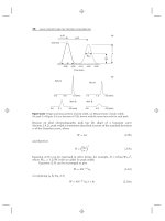
15.3.2 Touching-Peak Separation
Touching peak (T-P) separation was defined in Section 15.1.1. A weight of injected
sample is selected such that the broadened product peak just touches one of the two
surrounding peaks (as in Fig. 15.1b); this then allows a maximum weight of sample
for ≈100% recovery of the separated product in ≈100% purity. T-P separation can

be achieved by trial and error, guided by the following discussion.
If varying amounts of peak B in Figure 15.1 are injected, and the chro-
matograms superimposed, a series of so-called nesting right-triangles will result—as
in the illustration of Figure 15.5. Here, the three overloaded product peaks (1, 2, 4)
correspond to relative sample weights of 1, 2, and 4. The tail of each overloaded
peak is located near the retention time for a small weight of injected sample, and
for varying ‘‘small’’ weights of the sample there is no change in peak width (lin-
ear isotherm region; see Fig. 15.4b). The widths W of overloaded peaks increase
approximately in proportion to the square root of the sample weight (Eq. 15.4b). At
the bottom of Figure 15.5, a value of W is shown for the largest weight of injected
sample (peak 4), measured from the start of the peak at 6 minutes to the retention
time for a small sample (10 min). One way of determining the required weight of
injected sample for T-P separation is as follows: After an initial injection of a small
sample, an arbitrary increase in sample weight can be made for the next sample,
for example, resulting in curve 1 of Figure 15.5. In this case, W must be increased
740 PREPARATIVE SEPARATIONS
“small” samples
of varying weight
(t
R
= 10)
4
1
2
W
(p
eak 4
)
6 7 8 9 10 11 (min)
impurity

peak
product
peaks
Figure 15.5 Effect of sample weight on peak shape for overloaded separation (superimposed
chromatograms).
2-fold, to move the front of the product peak next to the adjacent impurity peak
(shaded). Since peak width increases as the square root of the sample weight, the
sample weight should therefore be increased 4-fold (4
0.5
= 2).
The weight of injected product for T-P separation depends on (1) the value of
the product separation factor α
0
for a small weight of injected sample, (2) the nature
of the sample, and (3) the saturation capacity of the column (Section 15.3.2.1). If
molecules of the product are not ionized, and a 10-nm-pore, 150 × 4.6-mm column
is assumed, the weight of injected product for T-P separation will be about 3 mg
for α
0
= 1.5. For columns differing in length or i.d., the latter product weight for
T-P separation will be proportional to the column internal volume. If α
0
equal 1.1
or 3.0, the corresponding sample weights will be about 0.2 and 10 mg, respectively.
The extent of sample ionization and column characteristics together determine the
column saturation capacity w
s
(see Section 15.3.2.1). The weight of injected product
w
x

for T-P separation can then be approximated by
w
x
=

1
6

α − 1
α

2
w
s
(15.5)
15.3.2.1 Column Saturation Capacity
An understanding of the column saturation capacity w
s
(which we will refer to
simply as ‘‘column capacity’’) is basic to any further discussion of prep-LC. The
value of w
s
corresponds to the maximum possible uptake of a solute molecule
by the column, that is, the weight of solute that will fill an adsorbed monolayer
completely (this corresponds to a large concentration of solute in the mobile phase);
see the hypothetical example of Figure 15.6a for the adsorption of benzene onto a
representative portion of the stationary-phase surface. Column capacity is specific to
a particular column and can vary somewhat with both the solute and experimental
15.3 ISOCRATIC ELUTION 741
(a)

(b)
mobile
phase
stationary
phase
mobile
phase
stationary
phase
NH
3
+
NH
3
+
NH
3
+
NH
3
+
NH
3
+
NH
3
+
NH
3
+

NH
3
+
NH
3
+
Figure 15.6 Illustration of column capacity as a function of solute ionization. Adsorption of
benzene (a) and protonated aniline (b).
conditions. The column capacity will be proportional to the accessible surface area
of the packing material, and for a non-ionized solute w
s
can be approximated by
w
s
(mg) = 0.4 (surface area in m
2
) (15.6)
While this might suggest the use of a column packing with the largest possible surface
area, higher surface packings have smaller diameter pores. If solute molecules are
large relative to the pore diameter, they cannot enter the pores and take full advantage
of the surface area (which is almost entirely contained within the pores) so that
the effective column capacity will be reduced. For large-pore packings, conversely,
the surface area and column capacity are both smaller. Thus intermediate pore-size
packings provide the largest column capacities (e.g., pore diameters of ≈8nmfor
solute molecular weights <500 Da); see the related discussion of Figure 13.7 for the
retention of larger molecules as a function of column pore diameter.
Some characteristics of the solute molecule (other than size) are also important.
Small solutes that adsorb perpendicular to the packing surface can result in a higher
column capacity than solutes which lie flat on the surface (compare Fig. 8.3b
with 8.3a). Large molecules, such as proteins, may assume a three-dimensional

742 PREPARATIVE SEPARATIONS
conformation when retained, resulting in a significantly greater thickness of the
adsorbed monolayer; in this case the saturation capacity can be much greater than
predicted by Equation (15.6)—as long as the pore diameter is large enough to
admit the protein molecule. Charged (ionized) solute molecules of the same kind will
repel each other when adsorbed, and this electrostatic repulsion can reduce column
capacity by as much as two orders of magnitude. This is illustrated in Figure 15.6,
where the uptake of a neutral solute (benzene) in Figure 15.6a is contrasted with
that of an ionized solute (protonated aniline) in Figure 15.6b. Because of the much
smaller column capacity for ionized solute molecules, prep-LC is preferably carried
out under conditions that minimize sample ionization. However, because of the
much greater retention of a non-ionized molecule vs. its ionized counterpart (e.g., a
nonprotonated base vs. the protonated base), partially ionized solutes should have
much larger column capacities than fully ionized species—if not as great as for
completely neutral molecules.
15.3.2.2 Sample-Volume Overload
The volume of the injected sample for a T-P separation depends on the required
product weight and the concentration of the product in the original sample solution
(which may be limited by sample solubility). It has been estimated [5] that the sample
volume will have little effect on prep-LC separation until the sample volume V
s
exceeds half the volume of the peak being collected; V
p
equals the peak width W times
the flow rate F. Figure 15.7 shows simulated chromatograms for a 0.1-mL injection
(solid line), a 1-mL injection (dotted line) and a 1.5-mL injection (dash-dotted line),
while holding the sample-weight constant by varying its concentration (values of
36 g/L, 3.6 g/L and 2.4 g/L, respectively). For the 1.5-mL sample volume, significant
peak overlap results, with only 85% recovery of pure peak A. It is clearly preferable
to use the highest possible sample concentration. For the lowest sample concentration

in Figure (15.7) (2.4 g/L), a T-P separation can only be achieved by reducing the
injection volume to less than 1 mL, with a consequent reduction in the weight of
pure A that can be recovered from each separation.
In order to avoid peak distortion and a deterioration of separation, as well
as other problems, it is usually best to use the same solvent composition for both
the sample and the mobile phase. However, sample solvents whose compositions
differ from that of the mobile phase may be required in order to improve sample
solubility (Section 15.3.2.3). Provided that the strength of the sample solvent and
mobile phase are similar, there should be little adverse effect on peak width or shape
from the use of a sample solvent and mobile phase that are not the same.
15.3.2.3 Sample Solubility
T-P separation requires a certain weight of the injected sample, preferably injected
in a volume of mobile phase that is less than
1
/
2
of the peak volume WF (as discussed
above). Sample solvents that are weaker than the mobile phase are acceptable, and
larger volumes of such sample solutions can be injected. However, sample solubility
often decreases when %B is reduced, so the injection of larger volumes of sample
dissolved in a weaker solvent may not provide a greater weight of injected sample.
Means of dealing with the problem of limiting sample solubility include:
15.3 ISOCRATIC ELUTION 743
0 2 4 6 8 10 12
(
min
)
V
s
(mL) =

0.1
1.0
1.5
A
Figure 15.7 Chromatograms illustrating the effects of volume overload on the separation of
two adjacent peaks. Sample volumes:____, 0.1 mL; , 1.0 mL; _ _ _, 1.5 mL. Simulation
for a column 250 × 4.6 mm operated at 1 mL/min, two components at 1:1 composition, k(A)
= 1.0, selectivity α = 1.5, N = 1000. The two peaks are moderately mass-overloaded.
• a change in the mobile phase
• a change in the sample solvent
• an increase in column temperature
Change in Mobile Phase. The choice of prep-LC mode (RPC or NPC) should
consider whether the sample is likely to be more soluble in aqueous solvents (RPC) or
in organic solvents (NPC). The choice of B-solvent in each case can further influence
sample solubility. On the other hand, the choice of mode and B-solvent also affects
selectivity α, so a compromise between mobile-phase solubility and selectivity may
be necessary when selecting the B-solvent.
Change in Sample Solvent. The sample solvent need not be the same as the
mobile phase but, generally, should not be much stronger. Just as the use of stronger
sample solvents adversely affects analytical separations (Sections 2.6.1, 17.4.5.3),
peak broadening and distortion can also occur in prep-LC separations when the
sample solvent is stronger than the mobile phase. Usually a sample solvent that
is similar in strength to the mobile phase will be the best choice. A change in
B-solvent for the sample solvent may improve solubility, especially for NPC where
sample solubility can be varied independently of solvent strength. Thus, the same
mobile-phase strength ε can be achieved with varying values of %B for different
B-solvents (see example of Fig. 8.6), depending on the polarity (or ε
0
value) of the
B-solvent. Since sample solubility is generally higher for a mobile phase with a higher

value of %B, this suggests the use of a sample solvent with as large a value of %B as
possible—while maintaining the same mobile-phase strength ε. For example, if the
mobile phase consists of 4% ethyl acetate in hexane, Figure 8.6 suggests the use of
50% CH
2
Cl
2
in hexane as a sample solvent that is likely to provide greater sample
solubility without adverse effects on the separation.
744 PREPARATIVE SEPARATIONS
Larger sample, bigger column,
higher flow
1. Initial separation
after adjusting %B
2. Maximize α for
product peak
3. Maximize
sample size
4. Scale up
d
a
b
c
d
(product)
e
b
c
a
e

Figure 15.8 Prep-LC method development.
A change in pH of the sample solvent is another option for increasing sample
solubility, when acidic or basic compounds are separated by RPC. In the latter case a
mobile-phase pH that suppresses sample ionization is usually preferred for increased
column capacity (as illustrated in Fig. 15.6), but sample solubility is often greater
for ionized compounds. This suggests the use of a sample-solvent pH that provides
increased sample ionization and solubility. Since an increase in solute ionization
decreases its retention (undesirable for a sample solvent), the sample solvent can be
lightly buffered, so that upon mixing with the mobile phase the resulting pH will be
similar to that of the mobile phase. However, this procedure assumes a relatively
small sample volume and a more heavily buffered mobile phase.
Whatever change in the sample solvent is considered, the possibility of sample
precipitation (with blockage of the injector, solvent tubing, or column) should
be kept in mind when the sample mixes with the mobile phase.Insomecases
precipitation may not occur instantaneously, allowing the sample to be taken up by
the column before precipitation can occur. Experiments where aliquots of sample
solution are mixed with the mobile phase and observed for a few minutes can
indicate the likelihood of precipitation problems during the separation (see the
related discussion of Section 7.2.1.2 for assessing buffer solubility). Alternatively,
the likelihood of sample precipitation when using a sample solvent different than
15.3 ISOCRATIC ELUTION 745
the mobile phase can be reduced by the technique of ‘‘at-column dilution’’ [7, 8].
The latter procedure introduces the sample via a separate pump to the head of the
column so that sample and mobile phase are mixed together just prior to entering
the column—with the likelihood that sample uptake by the stationary phase will
occur before sample precipitation.
Increase in Column Temperature. A temperature increase will generally increase
sample solubility, but the sample must also be heated during its passage from the
sample container to the column inlet (a sample pump can be a significant heat sink!).
A failure to heat any part of the system can lead to sample precipitation and blockage

of the injector, solvent tubing, or column. An increase in column temperature will
also reduce sample retention and may lead to smaller values of α —withanoffsetting
decrease in the weight of sample that can be injected.
15.3.2.4 Method Development
The development of a prep-LC separation is summarized in Figure 15.8; for steps
1 to 3 an analytical-scale column should be used (e.g., 150 × 4.6-mm). If a wider
column is required for an increase in the weight of purified sample from each run
(separation), this is selected in step 4.
Selection of Initial Conditions. Prior to Step-1 (initial separation), it is necessary
to choose either RPC or NPC, as well as select the initial separation conditions
(column type, mobile phase, temperature). Whereas RPC is generally favored for
analytical separations, NPC is often preferred for prep-LC—especially when the
sample is not water soluble and the required weight of purified product is more than
50 mg. We will assume NPC in the following discussion, but for the selection of
initial RPC conditions, see Chapters 6 and 7.
If more than 10 mg of purified product will be required, be sure that the same
column packing is available in larger-i.d. columns for scale-up (step 4). Next select
a strong (B) and weak (A) solvent for the mobile phase (see Chapter 8 for NPC;
e.g., ethyl acetate and hexane), and vary %B so that 1 ≤ k ≤ 10 for the product and
later-eluting peaks (if possible). Since peaks eluting before the product need not be
separated from each other, their values of k can be <1. Similarly, if some impurities
are strongly retained, they can be removed more quickly by washing the column
with a stronger mobile phase after elution of the product peak; the column must
then be equilibrated with the original mobile phase before injecting the next sample
(gradient elution is an alternative for such samples).
Step 1 of Figure 15.8. An initial separation is carried out next, using a similar
approach as for analytical method development, for example, using a strong mobile
phase (e.g., 80% B) in order to achieve the elution of the entire sample within a
reasonable time. The value of %B is next adjusted by trial and error to achieve 1
< k < 10 for the product peak, with lower values of k favored for faster separation

and the purification of a greater weight of product per hour (see Sections 2.5.1, 8.4).
Alternatively, thin-layer chromatography (Section 8.2.3) can be used for this pur-
pose, or an initial separation can be carried out using gradient elution—which
in turn allows an estimate of a preferred %B value for isocratic separation