The Illustrated Network- P48 pdf

the world over. ATM was part of an all-encompassing vision of networking known as
broadband ISDN (B-ISDN), which would support all types of voice, video, and data
applications though virtual channels (and virtual connections). In this model, the Inter-
net would yield to a global B-ISDN network—and TCP/IP to ATM.
Does this support plan for converged information sound familiar? Of course it does.
It’s pretty much what the Internet and TCP/IP do today, without B-ISDN or ATM. But
when ATM was fi rst proposed, the Internet and TCP/IP could do none of the things
that ATM was supposed to do with ease. How did ATM handle the problems of mixing
support for bulk data transfer with the needs of delay-sensitive voice and bandwidth-
hungry (and delay-sensitive) video?
ATM was the international standard for what was known as cell relay (there were
cell relay technologies other than ATM, now mostly forgotten). The cell relay name
seems to have developed out of an analogy with frame relay. Frame relay “relayed”
(switched) Layer 2 frames through network nodes instead of independently routing
Layer 3 packets. The effi ciency of doing it all at a lower layer made the frame relay node
faster than a router could have been at the time.
Cell relay took it a step further, doing everything at Layer 1 (the actual bit level).
But there was no natural data unit at the physical layer, just a stream of bits. So, they
invented one 53 bytes long and called it the “cell”—apparently in comparison to the
cell in the human body—which is very small, can be generic, and everything else is
built up from them. Technically, in data protocol stacks, cells are a “shim” layer slipped
between the bits and the frames, because both bits and frames are still needed in hard-
ware and software at source and destination.
Cell relay (ATM) “relayed” (switched) cells through network nodes. This could be
done entirely in hardware because cells were all exactly the same size. Imagine how
fast ATM switches would be compared to slow Layer 3 routers with two more layers
to deal with! And ATM switches had no need to allocate buffers in variable units, or to
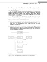
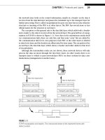
clean up fragmented memory. The structure of the 5-byte ATM cell header is shown in
Figure 17.4 (descriptions follow on next page). The call payload is always 48 bytes long.
GFC VPI
VCIVPI

VCI
VCI PTI CLP
HEC
8 Bits 1
UNI Cell Header
VPI
VCIVPI
VCI
VCI PTI CLP
HEC
8 Bits 1
NNI Cell Header
5
octets
FIGURE 17.4
The ATM cell header. Note the larger VPI fi elds on the network (NNI) version of the header.
CHAPTER 17 MPLS and IP Switching 439
■ GFC—The Generic Flow Control is a 4-bit fi eld used between a customer site and
ATM switch, on the User-Network Interface (UNI). It is not present on the Network–
Network Interface (NNI) between ATM switches.
■ VPI—The Virtual Path Identifi er is an 8- or 12-bit fi eld used to identify paths between
sites on the ATM network. It is larger on the NNI to accommodate aggregation on
customer paths.
■ VCI—The Virtual Connection Identifi er is a 16-bit fi eld used to identify paths between
individual devices on the ATM network.
■ PTI—The Payload Type Indicator is a 3-bit fi eld used to identify one of eight traffi c
types carried in the cell.
■ CLP—The Cell Loss Priority bit serves the same function as the DE bit in frame relay,
but identifi es cells to discard when congestion occurs.
■ HEC—The Header Error Control byte not only detects bit errors in the entire

40-bit header, but can also correct single bit errors.
In contrast to frame relay, the ATM connection identifi er was a two-part virtual path
identifi er (VPI) and virtual channel identifi er (VCI). Loosely, VPIs were for connections
between sites and VCIs were for connections between devices. ATM switches could
“route” cells based on the VPI, and the local ATM switch could take care of fi nding the
exact device for which the cell was destined.
Like frame relay DLCIs, ATM VPI/VCIs have local signifi cance only. That is, the VPI/
VPI values change as the cells make their way from switch to switch and depending on
direction. Both frame relay and ATM switch essentially take a data unit in on an input
port, look up the header (DLCI or VPI/VCI label) in a table, and output the data unit
on the port indicated in the table—but also with a new label value, also provided by
the table.
This distinctive label-swapping is characteristic of switching technologies and
protocols. And, as we will see later, switching has come to the IP world with MPLS,
which takes the best of frame relay and ATM and applies it directly to IP without the
burden of “legacy” stacks (frame relay) or phantom applications (ATM and B-ISDN).
The tiny 48-byte payload of the ATM cell was intentional. It made sure that no delay-
sensitive bits got stuck in a queue behind some monstrous chunk of data a thousand
times larger than the 48 voice or video bytes. Such “serialization delay” introduced
added delay and delay variation (jitter) that rendered converged voice and video almost
useless without more bandwidth than anyone could realistically afford. With ATM, all
data encountered was a slightly elevated delay when data cells shared the total band-
width with voice and video. But because few applications did anything with data (such
as a fi le) before the entire group of bits was transferred intact ATM pioneers deemed
this a minor inconvenience at worst.
All of this sounded too good to be true to a lot of networking people, and it turned
out that it was. The problem was not with raw voice and video, which could be molded
into any form necessary for transport across a network. The issue was with data, which
came inside IP packets and had to be broken down into 48-byte units—each of which
had a 5-byte ATM cell header, and often a footer that limited it to only 30 bytes.

440 PART III Routing and Routing Protocols
This was an enormous amount of overhead for data applications, which normally
added 3 or 4 bytes to an Ethernet frame for transport across a WAN. Naturally, no hard-
ware existed to convert data frames to cells and back—and software was much too
slow—so this equipment had to be invented. Early results seemed promising, although
the frame-to-cell-and-back process was much more complex and expensive than antici-
pated. But after ATM caught on, prices would drop and effi ciencies would be naturally
discovered. Once ATM networks were deployed, the B-ISDN applications that made the
most of them would appear. Or so it seemed.
However, by the early 1990s it turned out that making cells out of data frames was
effective as long as the bandwidth on the link used to carry both voice and video
along with the data was limited to less than that needed to carry all three at once.
In other words, if the link was limited to 50 Mbps and the voice and video data added
up to 75 Mbps, cells made sense. Otherwise, variable-length data units worked just fi ne.
Full-motion video was the killer at the time, with most television signals needing about
45 Mbps (and this was not even high-defi nition TV). Not only that, but it turned out that
the point of diminishing ATM returns (the link bandwidth at which it became slower
and more costly to make cells than simply send variable-length data units) was about
622 Mbps—lower than most had anticipated.
Of course, one major legacy of the Internet bubble was the underutilization of
fi ber optic links with more than 45 Mbps, and in many cases greatly in excess of
622 Mbps. And digital video could produce stunning images with less and less band-
width as time went on. And in that world, in many cases, ATM was left as a solution
without a problem. ATM did not suffer from lack of supporters, but it proved to be the
wrong technology to carry forward as a switching technology for IP networks.
Why Converge on TCP/IP?
Some of the general reasons TCP/IP has dominated the networking scene have been
mentioned in earlier chapters. Specifi cally, none of the “new” public network technolo-
gies were particularly TCP/IP friendly—and some seemed almost antagonistic. ATM
cells, for instance, would be a lot more TCP/IP friendly if the payload were 64 bytes

instead of 48 bytes. At least a lot of TCP/IP traffi c would fi t inside a single ATM cell
intact, making processing straightforward and effi cient.
At 48 bytes, everything in TCP/IP had to be broken up into at least two cells. But the
voice people wanted the cell to be 32 bytes or smaller, in order to keep voice delays as
short as possible. It may be only a coincidence that 48 bytes is halfway between 32 and
64 bytes, but a lot of times reaching a compromise instead of making a decision annoys
both parties and leaves neither satisfi ed with the result. So, ATM began as a standard
by alienating the two groups (voice and data) that were absolutely necessary to make
ATM a success.
But the real blow to ATM came because a lot of TCP/IP traffi c would not fi t into
64-byte frames. ACKs would fi t well, but TCP/IP packet sizes tend to follow a bimodal
distribution with two distinct peaks at about 64 and between 1210 and 1550 bytes.
The upper cluster is smaller and more spread out, but this represents the vast bulk of
all traffi c on the Internet.
CHAPTER 17 MPLS and IP Switching 441
Then new architectures allowed otherwise normal IP routers to act like frame relay
and ATM switches with the addition of IP-centric MPLS. Suddenly, all of the benefi ts
of frame relay and ATM could be had without using unfamiliar and special equipment
(although a router upgrade might be called for).
MPLS
Rather than adding IP to fast packet switching networks, such as frame relay and ATM,
MPLS adds fast packet switching to IP router networks. We’ve already talked about
some of the differences between routing (connectionless networks) and switching
networks in Chapter 13. Table 17.1 makes the same type of comparisons from a differ-
ent perspective.
The difference in the way CoS is handled is the major issue when convergence is
concerned. Naturally, the problem is to fi nd the voice and video packets in the midst of
the data packets and make sure that delay-sensitive packets are not fi ghting for bandwidth
along with bulk fi le transfers or email. This is challenging in IP routers because there is no
fi xed path set up through the network to make it easy to enforce QoS at every hop along

the way. But switching uses stable paths, which makes it easy to determine exactly which
routers and resources are consumed by the packet stream. QoS is also challenging because
you don’t have administrative control over the routers outside your own domain.
MPLS and Tunnels
Some observers do not apply the term “tunnel” to MPLS at all. They reserve the term
for wholesale violations on normal encapsulations (packet in frame in a packet, for
example). MPLS uses a special header (sometimes called a “shim” header) between
packet and frame header, a header that is not part of the usual TCP/IP suite layers.
However, RFCs (such as RFC 2547 and 4364) apply the tunnel terminology
to MPLS. MPLS headers certainly conform to general tunnel “rules” about stack
encapsulation violations. This chapter will not dwell on “MPLS tunnel” terminol-
ogy but will not avoid the term either. (This note also applies to MPLS-based VPNs,
discussed in Chapter 26.)
But QoS enforcement is not the only attraction of MPLS. There are at least two
others, and probably more. One is the ability to do traffi c engineering with MPLS, and
the other is that MPLS tunnels form the basis for a certain virtual private network
(VPN) scheme called Layer 3 VPNs. There are also Layer 2 VPNs, and we’ll look at them
in more detail in Chapter 26.
MPLS uses tunnels in the generic sense: The normal fl ow of the layers is altered at one
point or another, typically by the insertion of an “extra” header. This header is added at
one end router and removed (and processed) at the other end. In MPLS, routers form the
442 PART III Routing and Routing Protocols
endpoints of the tunnels. In MPLS, the header is called a label and is placed between the
IP header and the frame headers—making MPLS a kind of “Layer 2 and a half” protocol.
MPLS did not start out to be the answer to everyone’s dream for convergence or
traffi c engineering or anything else. MPLS addressed a simple problem faced by every
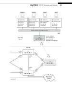
large ISP in the world, a problem shown in Figure 17.5.
MPLS was conceived as a sort of BGP “shortcut” connecting border routers across
the ISP. As shown in the fi gure, a packet bound for 10.10.100.0/24 entering the border
router from the upstream ISP is known, thanks to the IBGP information, to have to exit

the ISP at the other border router. In practice, of course, this will apply to many border
routers and thousands of routes (usually most of them), but the principle is the same.
Only the local packets with destinations within the ISP technically need to be
routed by the interior routers. Transit packets can be sent directly to the border router,
Table 17.1 Comparing Routing and Switching on a WAN
Characteristic Routing Switching
Network node Router Switch
Traffi c fl ow Each packet routed independently
hop by hop
Each data unit follows same
path through network
Node coordination Routing protocols share
information
Signaling protocols set up
paths through network
Addressing Global, unique Label, local signifi cance
Consistency of address Unchanged source to destination Label is swapped at each node
QoS Challenging Associated with path
Router
Router
Router
Router
ISP
Border
Router
Router
Router
Border
Router
Upstream

ISP
Downstream
ISP
Packet for
10.10.100.0/24
Network
10.10.100.0/24
(and many more)
FIGURE 17.5
The rationale for MPLS. The LSP forms a “shortcut” across the routing network for transit traffi c.
The Border Router knows right away, thanks to BGP, that the packet for 10.10.100.0/24 must exit
at the other border router. Why route it independently at every router in between?
CHAPTER 17 MPLS and IP Switching 443
if possible. MPLS provides this mechanism, which works with BGP to set up tunnels
through the ISP between the border routers (or anywhere else the ISP decides to use
them).
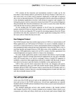
The structure of the label used in MPLS is shown in Figure 17.6. In the fi gure,
it is shown between a Layer 2 PPP frame and the Layer 3 IP packet (which is very
common).
■ Label—This 20-bit fi eld identifi es the packets included in the “fl ow” through the
MPLS tunnel.
■ CoS—Class-of-Service is a 3-bit fi eld used to classify the data stream into one of
eight categories.
■ S—The Stack bit lets the router know if another label is stacked after the
current 32-bit label.
■ TTL—The Time-to-Live is an 8-bit fi eld used in exactly the same way as the IP
packet header TTL. This value can be copied from or into the IP packet or used
in other ways.
Certain label values and ranges have been reserved for MPLS. These are outlined in
Table 17.2.

The MPLS architecture is defi ned in RFC 3031, and MPLS label stacking is defi ned in
RFC 3032 (more than one MPLS label can precede an IP packet). General traffi c engi-
neering in MPLS is described in RFC 2702, and several drafts add details and features
to these basics.
What does it mean to use traffi c engineering on a router network? Consider the
Illustrated Network. We saw that traffi c from LAN1 to LAN2 fl ows through backbone
routers P4 and P2 (reverse traffi c also fl ows this way). But notice that P2 and P4 also
have links to and from the Internet. A lot of general Internet traffi c fl ows through rout-
ers P2 and P4 and their links, as well as LAN1 and LAN2 traffi c.
PPP Header
MPLS Label
(32 bits)
IP Packet
Label
20 bits 3 bits 1
bit
8 bits
CoS S TTL
FIGURE 17.6
The 32-bit MPLS label fi elds. Note the 3-bit CoS fi eld, which is often related to the IP ToS header.
The label fi eld is used to identify fl ows that should be kept together as they cross the network.
444 PART III Routing and Routing Protocols
So, it would make sense to “split off” the LAN1 and LAN2 traffi c onto a less utilized
path through the network (for example, from PE5 to P9 to P7 to PE1). This will ease
congestion and might even be faster, even though in some confi gurations there might
be more hops (for example, there might be other routers between P9 and P7).
Table 17.2 MPLS Label Values and Their Uses
Value or Range Use
0 IPv4 Explicit Null. Must be the last label (no stacking). Receiver
removes the label and routes the IPv4 packet inside.

1 Router Alert. The IP packet inside has information for the
router itself, and the packet should not be forwarded.
2 IPv6 Explicit Null. Same as label 0, but with IPv6 inside.
3 Implicit Null. A “virtual” label that never appears in the
label itself. It is a table entry to request label removal by the
downstream router.
4–15 Reserved.
16–1023 and 10000–99999 Ranges used in Juniper Networks routers to manually confi gure
MPLS tunnels (not used by the signaling protocols).
1024–9999 Reserved.
100000–1048575 Used by signaling protocols.
Why Not Include CE0 and CE6?
Why did we start the MPLS tunnels at the provider-edge routers instead of directly
at the customer edge, on the premises? Actually, as long as the (generally) smaller
site routers support the full suite of MPLS features and protocols there’s no reason
the tunnel could not span LAN to LAN.
However, MPLS traditionally begins and ends in the “provider cloud”—usually
on the PE routers, as in this chapter. This allows the customer routers to be more
independent and less costly, and allows reconfi guration of MPLS without access to
the customer’s routers. Of course, in some cases the customer might want ISP to
handle MPLS management—and then the CE routers certainly could be included
on the MPLS path.
There are ways to do this with IGPs, such as OSPF and IS–IS, by adjusting the link
metrics, but these solutions are not absolute and have global effects on the network.
In contrast, an MPLS tunnel can be confi gured from PE5 to PE1 through P9 and P7 and
CHAPTER 17 MPLS and IP Switching 445
only affect the routing on PE5 and PE1 that involves LAN1 and LAN2 traffi c, exactly the
effect that is desired.
MPLS Terminology
Before looking at how MPLS would handle a packet sent from LAN1 to LAN2 over an

MPLS tunnel, we should look at the special terminology involved with MPLS. In no
particular order, the important terms are:
LSP—We’ve been calling them tunnels, and they are, but in MPLS the tunnel is
called a label-switched path. The LSP is a unidirectional connection following
the same path through the network.
Ingress router—The ingress router is the start of the LSP and where the label is
pushed onto the packet.
Egress router—The egress router is the end of the LSP and where the label is
popped off the packet.
Transit or intermediate router—There must be at least one transit (sometimes
called intermediate) router between ingress and egress routers. The transit
router(s) swaps labels and replaces the incoming values with the outgoing
values.
Static LSPs—These are LSPs set up by hand, much like permanent virtual circuits
(PVCs) in FR and ATM. They are difficult to change rapidly.
Signaled LSPs—These are LSPs set up by a signaling protocol used with MPLS
(there are two) and are similar to switched-virtual circuits (SVCs) in FR
and ATM.
MPLS domain—The collection of routers within a routing domain that starts and
ends all LSPs form the MPLS domain. MPLS domains can be nested, and can be
a subset of the routing domain itself (that is, all routers do not have to under-
stand MPLS; only those on the LSP).
Push, pop, and swap—A push adds a label to an IP packet or another MPLS label.
A pop removes and processes a label from an IP packet or another MPLS label.
A swap is a pop followed by a push and replaces one label by another (with
different field values). Multiple labels can be added (push push . . .) or removed
(pop pop . . .) at the same time.
Penultimate hop popping (PHP)—Many of LSPs can terminate at the same bor-
der router. This router must not only pop and process all the labels but route
all packets inside, plus all other packets that arrive from within the ISP. To

ease the load of this border router, the router one hop upstream from the
egress router (known as the penultimate router) can pop the label and simply
route the packet to the egress router (it must be one hop, so the effect is the
446 PART III Routing and Routing Protocols
same). PHP is an optional feature of LSPs, and keep in mind that the LSP is still
considered to terminate at the egress router (not at the penultimate).
Constrained path LSPs—These are traffic engineering (TE) LSPs set up by a
signaling protocol that must respect certain TE constraints imposed on the
network with regard to delay, security, and so on. TE is the most intriguing
aspect of MPLS.
IGP shortcuts—Usually, LSPs are used in special router tables and only available to
routes learned by BGP (transit traffic). Interior Gateway Protocol (IGP) short-
cuts allow LSPs to be installed in the main routing table and used by traffic
within the ISP itself, routes learned by OSPF or another IGP.
Signaling and MPLS
There are two signaling protocols that can be used in MPLS to automatically set up
LSPs without human intervention (other than confi guring the signaling protocols
themselves!). The Resource Reservation Protocol (RSVP) was originally invented to set
up QoS “paths” from host to host through a router network, but it never scaled well or
worked as advertised. Today, RSVP has been defi ned in RFC 3209 as RSVP for TE and is
used as a signaling protocol for MPLS. RSVP is used almost exclusively as RSVP-TE (most
people just say RSVP) by routers to set up LSPs (explicit-path LSPs), but can still be used
for QoS purposes (constrained-path LSPs).
The Label Distribution Protocol (LDP), defi ned in RFC 3212, is used exclusively with
MPLS but cannot be used for adding QoS to LSPs other than using simple constraints
when setting up paths. On the other hand, LDP is trivial to confi gure compared to RSVP.
This is because LDP works directly from the tables created by the IGP (OSPF or IS–IS).
The lack of QoS support in LDP is due to the lack of any intention in the process. The
reason for the LDP paths created from the IGP table to exist is only simple adjacency. In
addition, LDP does not offer much if your routing platform can forward packets almost

as fast as it can switch labels. Today, use of LDP is deprecated (see the admonitions in
RFC 3468) in favor of RSVP-TE.
A lot of TCP/IP texts spend a lot of time explaining how RSVP-TE works (they deal
with LDP less often). This is more of an artifact of the original use of RSVP as a host-
based protocol. It is enough to note that RSVP messages are exchanged between all
routers along the LSP from ingress to egress. The LSP label values are determined, and
TE constraints respected, hop by hop through the network until the LSP is ready for
traffi c. The process is quick and effi cient, but there are few parameters that can be
confi gured even on routers that change RSVP operation signifi cantly (such as interval
timers)—and none at all on hosts.
Although not discussed in detail in this introduction to MPLS, another protocol is
commonly used for MPLS signaling, as described in RFC 2547bis. BGP is a routing pro-
tocol, not a signaling protocol, but the extensions used in multiprotocol BPG (MPBGP)
make it well suited for the types of path setup tasks described in this chapter. With
MPBGP, it is possible to deploy BGP- and MPLS-based VPNs without the use of any other
CHAPTER 17 MPLS and IP Switching 447
signaling protocol. LSPs are established based on the routing information distributed by
MPBGP from PE to PE. MPBGP is backward compatible with “normal” BGP, and thus use
of these extensions does not require a wholesale upgrade of all routers at once.
Label Stacking
Of all the MPLS terms outlined in the previous section, the one that is essential to
understand is the concept of “nested” LSPs; that is, LSPs which include one or more
other LSPs along their path from ingress to egress. When this happens, there will be
more than one label in front of the IP packet for at least part of its journey.
It is common for many large ISPs to stack three labels in front of an IP packet. Often,
the end of two LSPs is at the same router and two labels are pushed or popped at once.
The current limit is eight labels.
There are several instances where this stacking ability comes in handy. A larger ISP
can buy a smaller ISP and simply “add” their own LSPs onto (outside) the existing ones.
In addition, when different signaling protocols are used in core routers and border

routers, these domains can be nested instead of discarding one or the other.
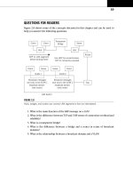
The general idea of nested MPLS domains with label stacking is shown in Figure 17.7.
There are fi ve MPLS domains, each with its own way of setting up LSPs: static, RSVP,
and LDP. The fi gure shows the number of labels stacked at each point and the order
R R R R
MPLS Domain 1
MPLS Domain 2
MPLS Domain 3
Static RSVP
RSVP
MPLS
Domain 4
LDP
MPLS
Domain 5
LDP
Two stacked labels
(MPLS2, MPLS1, IP)
Three stacked labels
(MPLS4, MPLS3,
MPLS1, IP)
Three stacked labels
(MPLS5, MPLS3,
MPLS1, IP)
FIGURE 17.7
MPLS domains, showing how the domains can be nested or chained, and how multiple labels
are used.
448 PART III Routing and Routing Protocols