signal processing for mobile communications handbook - crc press - 2005

CRC PRESS
w York Washington, D.C.
HANDBOOK
Edited by
Mohamed Ibnkahla
SIGNAL PROCESSING FOR
MOBILE COMMUNICATIONS
This book contains information obtained from authentic and highly regarded sources. Reprinted material is quoted with
permission, and sources are indicated. A wide variety of references are listed. Reasonable efforts have been made to publish
reliable data and information, but the authors and the publisher cannot assume responsibility for the validity of all materials
or for the consequences of their use.
Neither this book nor any part may be reproduced or transmitted in any form or by any means, electronic or mechanical,
including photocopying, microfilming, and recording, or by any information storage or retrieval system, without prior
permission in writing from the publisher.
All rights reserved. Authorization to photocopy items for internal or personal use, or the personal or internal use of specific
clients, may be granted by CRC Press LLC, provided that $1.50 per page photocopied is paid directly to Copyright Clearance
Center, 222 Rosewood Drive, Danvers, MA 01923 USA The fee code for users of the Transactional Reporting Service is
ISBN 0-8493-1657-X/05/$0.00+$1.50. The fee is subject to change without notice. For organizations that have been granted
a photocopy license by the CCC, a separate system of payment has been arranged.
The consent of CRC Press LLC does not extend to copying for general distribution, for promotion, for creating new works,
or for resale. Specific permission must be obtained in writing from CRC Press LLC for such copying.
Direct all inquiries to CRC Press LLC, 2000 N.W. Corporate Blvd., Boca Raton, Florida 33431.
Trademark Notice: Product or corporate names may be trademarks or registered trademarks, and are used only for
identification and explanation, without intent to infringe.
Visit the CRC Press Web site at www.crcpress.com
© 2005 by CRC Press LLC
No claim to original U.S. Government works
International Standard Book Number 0-8493-1657-X
Library of Congress Card Number 2004042812
America 1 2 3 4 5 6 7 8 9 0

Printed on acid-free paper
Library of Congress Cataloging-in-Publication Data
Signal processing for mobile communications handbook / edited by Mohamed Ibnkahla.
p. cm.
Includes bibliographical references and index.
ISBN 0-8493-1657-X (alk. paper)
1. Signal processing. 2. Mobile communication systems. I. Ibnkahla, Mohamed.
TK5102.9.S5427 2004
621.382′2—dc22 2004042812
Preface
Signal processing (SP) is a key research area in mobile communications. The recent years have known a real
explosion in research addressing different aspects of mobile communications signal processing. This area
is continuously expanding with emerging applications and services such as interactive multimedia and
Internet. SP has to meet the new challenges presented to future mobile communication systems such as
very low bit error rates, very high transmission rates, real-time multimedia access, and differential quality
of service (QoS).
Today’s publications in this area are scattered worldwide across multiple journals and conference pro-
ceedings. Like any other discipline that seeksto reach maturity, now is the time for mobile communications
signal processing to be presented to the readers in a comprehensive way and in one single book that stands
by itself. This book brings together most SP techniques, delivering, for the first time in the history of SP,
an in-depth survey of these techniques in a tutorial style.
The book is supported with more than 300 figures and tables, which makes it very easy to understand
and accessible to students, researchers, professors, engineers, managers, and any professional involved in
mobile communications.
The book investigates classical SP areas such as adaptive equalization, channel modeling and identifi-
cation, multi-user detection, and array processing. It also investigates newer areas such as adaptive coded
modulation, multiple-input multiple-output (MIMO) systems, diversity combining, and time-frequency
analysis. It explores emerging techniques such as neural networks, Monte Carlo Markov Chain (MCMC)
methods, and Chaos. It offers an excellent tutorial survey of promising approaches for future mobile
communications such as cross-layer design in multi-access networks and adaptive wireless networks.

In addition to wireless terrestrial communications, the book covers most applications areas of mobile
communications signal processing, such as satellite mobile communications, networking, power control
and resource management, voice over IP, positioning and geolocation, cross-layer design and adaptation,
etc.
I thank all the contributors for their excellent work. Thanks also to my research group at Queen’s
University who have dynamically contributed in writing three chapters and in the review process. Many
thanks to the different reviewers (about 80) whose valuable input, remarks, and suggestions have definitely
improved the technical quality of the chapters.
A special thank you to my wife, my son, and our families who have been a great support since the
beginning until the final stage of this project.
Mohamed Ibnkahla
Queen’s University
Kingston, Ontario, Canada
Editor
Mohamed Ibnkahla obtained an engineering degree in electronics in 1992, an M.Sc. degree in signal and
image processing in 1992, a Ph.D. degree in signal processing in 1996, and an HDR (the ability to lead and
supervise research) degree in digital communications and signal processing in 1998, all from the National
Polytechnic Institute of Toulouse (INPT), Toulouse, France.
Dr. Ibnkahla held an Assistant Professorship at INPT (1996–1999). In 2000, he joined the Department
of Electrical and Computer Engineering at Queen’s University, Kingston, Ontario, Canada as Assistant
Professor. He now holds the position of Associate Professor in the same department.
Since 1996, Dr. Ibnkahla has been involved in several research programs and centers of excellence, such
as the European Advanced Communications Technologies and Services Program (ACTS), Communica-
tions and Information Technology Ontario (CITO), Canadian Institute for Telecommunications Research
(CITR), and others. He has published a significant number of refereed journal papers, book chapters, and
conference papers.
His research interests include signal processing, mobile communications, digital communications, satel-
lite communications, and adaptive systems.
Dr. Ibnkahla received the INPT Leopold Escande Medal for the year 1997, France, for his research
contributions to signal processing, and the prestigious Premier’s Research Excellence Award (PREA),

Ontario, December 2000, for his contributions in wireless mobile communications.
Contributors
Karim Abed-Meraim
Ecole Nationale Superieure des
Telecommunications
Paris, France
Andreas Abel
ITI GmbH
Dresden, Germany
Hisham Abdul Hussein
Al-Asady
Queen’s University
Kingston, Ontario, Canada
Naofal Al-Dhahir
The University of Texas
Dallas, Texas
Mohamed-Slim Alouini
University of Minnesota
Minneapolis, Minnesota
Moeness Amin
Villanova University
Villanova, Pennsylvania
Hüseyin Arslan
University of South Florida
Tampa, Florida
Ghazem Azemi
Queensland University
Brisbane, Queensland,
Australia
Nicholas Bambos

A. Belouchrani
Ecole Nationale Polytechnique
Algeria
Boualem Boashash
Queensland University
Brisbane, Queensland,
Australia
Helmut Bölcskei
Swiss Federal Institute of
Technology (ETH)
Zurich, Switzerland
Rober Boutros
Queen’s University
Kingston, Ontario, Canada
Stefano Buzzi
University of Cassino
Cassino, Italy
James J. Caffery, Jr.
University of Cincinnati
Cincinnati, Ohio
Giovanni Cherubini
IBM Research
Zurich, Switzerland
Giovanni E. Corazza
University of Bologna
Bologna, Italy
Fernando D
´
ıaz-De-Mar
´

ıa
University of Carlos III
Inbar Fijalkow
Universit
´
e de Cergy Pontoise
Pontoise, France
Ascensio Gallardo-Antolin
University of Carlos III
de Madrid
Madrid, Spain
Mounir Ghogho
University of Leeds
Leeds, England
Filippo Giannetti
University of Pisa
Pisa, Italy
Savvas Gitzenis
Stanford University
Stanford, California
Dennis L. Goeckel
University of Massachusetts
Amherst, Massachusetts
Mohamed Ibnkahla
Queen’s University
Kingston, Ontario,
Canada
Ming Kang
University of Minnesota
Minneapolis, Minnesota

Geert Leus
Delft University
The Netherlands
Alan Lindsey
U.S. Air Force Research Lab
Remsen, New York
Nguyen Linh-Trung
Aston University
Birmingham, England
Marco Luise
University of Pisa
Pisa, Italy
Andreas F. Molisch
Lund University
Lund, Sweden
and
Mitsubishi Electric
Research Labs
Cambridge, Massachusetts
Marc Moonen
Katholieke Universiteit Leuven
Leuven, Belgium
Massimo Neri
University of Bologna
Bologna, Italy
Raffaella Pedone
University of Bologna
Bologna, Italy
Carmen Pel
´

aez-Moreno
Universidad Carlos III
de Madrid
Madrid, Spain
Quazi Mehbubar Rahman
Queen’s University
Kingston, Ontario, Canada
Atul Salhotra
Cornell University
Ithaca, New York
Anna Scaglione
Cornell University
Ithaca, New York
Wolfgang Schwarz
Dresden University of
Technology
Dresden, Germany
Noura Sellami
Universit
´
e de Cergy Pontoise
Pontoise, France
Bouchra Senadji
Queensland University
Brisbane, Queensland,
Australia
Mohamed Siala
Sup’Com
El Ghazaia Ariana,
Tunisia

We i S u n
Villanova University
Villanova, Pennsylvania
Ananthram Swami
U.S. Army Research Laboratory
Adelphi, Maryland
Lang Tong
Cornell University
Ithaca, New York
Fredrik Tufvesson
Lund University
Lund, Sweden
Jitendra K. Tugnait
Auburn University
Auburn, Alabama
Alessandro Vanelli-Coralli
University of Bologna
Bologna, Italy
Saipradeep Venkatraman
University of Cincinnati
Cincinnati, Ohio
Azadeh Vosoughi
Cornell University
Ithaca, New York
Xiaodong Wang
Columbia University
New York, New York
Hong-Chuan Yang
University of Victoria
Victoria, British Colombia,

Canada
Jun Yuan
Queen’s University
Kingston, Ontario,
Canada
Qing Zhao
Cornell University
Ithaca, New York
Contents
Part I: Introduction
1 Signal Processing for Future Mobile Communications Systems: Challenges
and Perspectives
Part II: Channel Modeling and Estimation
2 Multipath Propagation Models for Broadband Wireless Systems
3 Modeling and Estimation of Mobile Channels
4
Mobile Satellite Channels: Statistical Models and Performance Analysis
5
Mobile Velocity Estimation for Wireless Communications
Part III: Modulation Techniques for Wireless Communications
6 Adaptive Coded Modulation for Transmission over Fading Channels
7 Signaling Constellations for Transmission over Nonlinear Channels
8 Carrier Frequency Synchronization for OFDM Systems
9 Filter-Bank Modulation Techniques for Transmission over Frequency-Selective
Channels
Part IV: Multiple Access Techniques
10 Spread-Spectrum Techniques for Mobile Communications
11 Multiuser Detection for Fading Channels
Part V: MIMO Systems
12 Principles of MIMO-OFDM Wireless Systems

13 Space–Time Coding and Signal Processing for Broadband Wireless
Communications
14 Linear Precoding for MIMO Systems
15
Performance Analysis of Multiple Antenna Systems
Part VI: Equalization and Receiver Design
16 Equalization Techniques for Fading Channels
17 Low-Complexity Diversity Combining Schemes for Mobile
Communications
18 Overview of Equalization Techniques for MIMO
Fading Channels
19 Neural Networks for Transmission over Nonlinear Channels
Part VII: Voice over IP
20 Voice over IP and Wireless: Principles and Challenges
Part VIII: Wireless Geolocation Techniques
21 Geolocation Techniques for Mobile Radio Systems
22 Adaptive Arrays for GPS Receivers
Part IX: Power Control and Wireless Networking
23 Transmitter Power Control in Wireless Networking: Basic Principles
and Core Algorithms
24 Signal Processing for Multiaccess Communication Networks
Part X: Emerging Techniques and Applications
25 Time–Frequency Signal Processing for Wireless Communications
26 Monte Carlo Signal Processing for Digital Communications: Principles
and Applications
27 Principles of Chaos Communications
28
Adaptation Techniques and Enabling Parameter Estimation Algorithms
for Wireless Communications Systems
1

Signal Processing for
Future Mobile
Communications
Systems: Challenges
and Perspectives
Quazi Mehbubar Rahman
Queen’s University
Mohamed Ibnkahla
Queen’s University
1.1 Introduction
1.2 Channel Characterizations
Large-Scale Propagation Models
•
Small-Scale Propagation
Models
1.3 Modulation Techniques
Modulation Schemes: The Classification
•
Different Modulation Schemes
1.4 Coding Techniques
Shannon’s Capacity Theorem
•
Different Coding Schemes
•
Coding in Next-Generation Mobile Communications:
Some Research Evidence and Challenges
1.5 Multiple Access Techniques
Fundamental Multiple-Access Schemes
•
Combination

of OFDM and CDMA Systems
•
OFDM/TDMA
•
Capacity
of MAC Methods
•
Challenges in the MAC Schemes
1.6 Diversity Technique
Classifications of the Diversity Techniques
•
Classifications
of Diversity Combiners
•
Diversity for Next-Generation
Systems: Some Research Evidence
•
Challenges in the
Diversity Area
1.7 Conclusions
Abstract
This chapter briefly reviewsbackground information ondifferentsignal processing issues of wirelessmobile
communications systems targeting the next-generation scenarios. The overview includes the channel
characterization at the beginning of the chapter and then it steps through modulation techniques, multiple
access schemes, coding, and diversity techniques. Here, along with the presentation of current research
evidence, key challenges for the next-generation systems have been addressed.
Copyright © 2005 by CRC Press LLC
1.1 Introduction
The ability to communicate on the move has evolved remarkably since Guglielmo Marconi first demon-
strated radio’s ability to provide continuous contact with ships sailing the English Channel. That was

in 1897, and since then people throughout the world have enthusiastically adopted new wireless com-
munications methods and services. Currently, when the telecommunications industries are deploying
third-generation (3G) systems worldwide and researchers are presenting many new ideas for the next-
generation wireless systems (termed 4G), several challenges are yet to be fulfilled. These include high data
rate transmissions(up to 1 Gbps),multimediacommunications,seamless global roaming,quality of service
(QoS) management, high user capacity, integration and compatibility between 3G and next-generation
components, etc. To meet these challenges, researchers are presently focusing their attentions on different
signal processing issues after careful channel characterizations. This chapter will provide brief background
information on these issues. It will also include some information on the current research works and
challenges in these areas. The outline of the chapter follows: Section 1.2 discusses basic information on the
channel characterization aspects. Section 1.3 presents an overview of the different modulation schemes
that are getting the most attention in the research area. Coding techniques are discussed in Section 1.4.
Section 1.5 talks about different multiple access schemes, while Section 1.6 presents different diversity
scenarios. Finally, conclusions are drawn.
1.2 Channel Characterizations
The time-varying nature of the wireless mobile channel makes channel characterization and its analysis an
important issue. In a mobile wireless scenario, thetime-varying nature ofthe channel could be encountered
in many different ways, e.g., a relative motion between the transmitter and the receiver, time variation in
the structure of the medium, etc. All these scenarios make the channel characteristics random, and do
not offer any easy analysis on the signals, transmitted through this channel. In general, as an information
signal propagates through the channel, the strength of this signal decreases as the distance between the
transmitter and receiver increases. The strength of the received signal depends on the characteristics of the
channel and on the distance between the transmitter and the receiver. In a broad sense, the channel can be
modeled in two different categories, large-scale propagation model and small-scale propagation model.
These models will be discussed in the following subsections.
1.2.1 Large-Scale Propagation Models
Large-scale propagation model characterizes the received signal strength over large transmitter–receiver
separation distances of several hundreds or thousands of meters. These are broadly classified in to two cate-
gories: deterministic and stochastic. Both deterministic and stochastic approaches are useful in describing
a time-varying channel, even though they embrace different aspects: the stochastic model is better suited

for describing global behaviors, whereas the deterministic one is more useful for studying the transmission
through a specific channel realization.
1.2.1.1 Deterministic Approach
1.2.1.1.1 Free-Space Propagation Model
According to this model, the received signal power decays as a function of the distance between the
transmitter and the receiver when they maintain a clear line of sight between them. In this case, the free-
space signal power P
r
(d), received by a receiver antenna at a distance d (meters) from the transmitter, is
given by
P
r
(
d
)
=
P
t
G
t
G
r
λ
2
(
4π
)
2
d
2

L
, d ≥ d
0
(
= 0
)
≥ d
f
(1.1)
Copyright © 2005 by CRC Press LLC
TABLE 1.1 Path Loss Exponent for Different
Communication Environments
Communication Environment Path Loss Exponent
Indoor with line of sight 1.6–1.8
Free space 2
In factories with obstructions 2–3
Cellular radio in the urban area 2.7–3.5
Cellular radio in the shadowed urban area 3–5
Indoor with obstructions 4–6
where P
t
represents the transmitted signal power, G
t
andG
r
are the transmitter and receiver antenna
gains, respectively, L (≥1) is the system loss factor, independent of signal propagation, λ (meters) is the
wavelength, d
f
is the far-field distance (also known as Fraunhofer distance), and d

0
is the received-power
reference distance. The far-field distance d
f
is given by
d
f
=
2D
2
λ
d
f
>> D (1.2)
where D is the largest physical linear dimension of the antenna. Using Equation 1.1, the free-space received
power at a distance d > d
0
can be written as
P
r
(d) = P
r
(d
0
)

d
d
0


−2
(1.3)
1.2.1.1.2 Log-Distance Path Loss Model
This model showsthat the averagepathloss
1
increaseslogarithmically withdistance between the transmitter
and the receiver of a communications system, which is given by
Pl
avg
(
dB
)
= Pl
avg
(
d
0
)
+ 10n log

d
d
0

(1.4)
where n is the path loss exponent that indicates the rate at which the path loss for the transmitted signal
increases with distance. The value of n depends on the specific propagation environment (e.g., see Table 1.1
[Rap96]). In Equation 1.4, d and d
0
hold the same definitions as in Equation 1.1.

1.2.1.2 Stochastic Approach
1.2.1.2.1 Lognormal Shadowing Model
The phenomenon that describes the random shadowing effects occurring over a large number of mea-
surement locations having the same transmitter and receiver separation with different levels of clutter on
the propagation path is referred to as lognormal shadowing. The corresponding path loss model states
that the path loss Pl(d) at a particular location is lognormally (normal in dB) distributed about the mean
distance-dependent value [Cox84] [Ber87]. The analytical expression of this model is given by
Pl(d) = Pl
avg
(d) + X
σ
= Pl
avg
(d
0
) +10n log

d
d
0

+ X
σ
(1.5)
where X
σ
(dB) is a zero-mean Gaussian distributed random variable with a variance of σ
2
dB. In gen-
eral, the values of n (defined earlier) and σ

2
are computed from measured data (e.g., see Table 3.6 in
1
Path loss, expressed in dB, is defined as the difference between the effective transmitted signal power and the
received signal power.
Copyright © 2005 by CRC Press LLC
Rappaport [Rap96]), using linear regression in such a way that the contrast between the estimated and
measured path losses is minimized.
Other than the general large-scale propagation models described above, there are some specific models
based on the outdoor and indoor environments separately. These channel models are based on the profile
of the particular area. Examples of some outdoor propagation models include the Longley–Rice model
[Lon68] and Durkin’s model [Dad75]. Examples of some indoor models are the Erricson multiple break-
point model [Ake88] and the attenuation factor model [Sei92]. In addition to these models, Ray tracing
and site-specific modeling techniques are also used for both outdoor and indoor environments.
1.2.2 Small-Scale Propagation Models
These models characterize the received signal strength of a radio signal over a short period of time or travel
distance of typically 5λ to 40λ, λ being the wavelength of the signal. In this scenario, the instantaneous
received signal fluctuates very rapidly and may give rise to fading, which is termed small-scale fading.
In this section we will discuss different small-scale propagation models upon presenting all the relevant
parameters that are required to discuss these models.
1.2.2.1 Parameters of Mobile Multipath Channel
A multipath channel is characterized by many important parameters. Among these parameters delay
spread and coherence bandwidth describe the time-dispersive nature of the channel in a local area. On the
other hand, Doppler spread and coherence bandwidth describe the time-varying nature of the channel in a
small-scale region. Including these major parameters, here we will briefly discuss the channel parameters,
which will provide a clear description of a mobile multipath channel.
1.2.2.1.1 Fading
Fading, also known as small-scale fading, is the result of interference between two or more attenuated
versions of the transmitted signal arriving at the receiver in such a way that these signals are added
destructively. These multiple versions of the transmitted signal result from the multiple paths present in

the channel or from the rapid dynamic changes of the channel. In this case, the speed of the mobile and
the transmission bandwidth of the signal also play a vital role.
1.2.2.1.2 Doppler Shift
The apparent change in frequency of the transmitted signal due to the relative motion of the mobile is
known as the Doppler shift, which is given by
f
ds
=
v
λ
cos θ
(1.6)
where v is the velocity of the mobile, λ is the signal wavelength, and θ is the spatial angle between the
direction of motion of the mobile and the direction of arrival of the wave.
1.2.2.1.3 Excess Delay
This is the relative delay of the i th multipath signal component, compared to the first arriving component
and is given by τ
i
.
1.2.2.1.4 Power Delay Profile, Φ
c
(τ )
This is the average output signal power of the channel as a function of excess time delay τ.Inpractice,
c
(τ )
is measured by transmitting very narrow pulses, or equivalently a wide band signal, and cross-correlating
the received signal with a delayed version of itself. Power delay profile is also known as multipath intensity
profile and delay power spectrum. It gets the latter name because of its frequency domain component,
which gives the power spectrum density. The mean excess delay, root mean squared (rms) delay spread,
and excess delay spread (XdB) are multipath channel parameters that can be determined from a power

delay profile. The mean excess delay (τ
mean
) is the first moment of the power delay profile, the rms delay
Copyright © 2005 by CRC Press LLC
spread (σ
τ
) is the square root of the second central moment of the power delay profile, and the maximum
excess delay (XdB) of the power delay profile is defined as the time delay during which multipath energy
falls to X dB below the maximum value. τ
mean
and σ
τ
are expressed as
τ
mean
=

i
P (τ
i
)τ
i

i
P (τ
i
)
and
(1.7a)
σ

τ
=

mean[(τ )
2
] −τ
2
mean
(1.7b)
where
mean[(τ )
2
] =

i
P (τ
i
)τ
2
i

i
P (τ
i
)
(1.7c)
1.2.2.1.5 Delay Spread (T
m
)
Delay spread, also known as multipath spread, of the channel is the range of values of excess time delay τ ,

over which 
c
(τ ) is essentially nonzero.
1.2.2.1.6 Coherence Bandwidth (BW
coh
)
The frequency band in which all the spectral components of the transmitted signal pass through a channel
with equal gain and linear phase is known as coherence bandwidth of that channel. Over this bandwidth
the channel remains invariant. BW
coh
can be expressed in terms of rms delay spread, though there is no
exact relationship between these two parameters. According to Lee [Lee89], with a frequency correlation
of approximately 90%, BW
coh
can be shown as
BW
coh
≈
1
50σ
τ
(1.8)
1.2.2.1.7 Doppler Spread (B
d
)
Spreading of the frequency spectrum of the transmitted signal resulting from the rate of change of the
mobile radio channel is known as Doppler spread. With the transmitted signal frequency f
c
, the resultant
Doppler spectrum has the components in the range between ( f

c
− f
d,max
) and ( f
c
+ f
d,max
), f
d,max
being
the maximum Doppler frequency shift.
1.2.2.1.8 Coherence Time (T
coh
)
The time period during which the channel impulse response remains invariant is known as coherence
time of the channel. T
coh
is inversely proportional to the Doppler spread, and with the maximum Doppler
frequency shift, f
d,max
,itisgivenby
T
coh
≈
1
f
d,max
(1.9)
1.2.2.2 Types of Small-Scale Fading
Small-scale fading is divided into two broad classes, which are based on the time delay spread and Doppler

spread. The time delay spread-dependent class is divided into two categories, flat fading and frequency-
selective fading, while the Doppler spread-dependent class is categorized as fast and slow fading. It is
important to note that fast and slow fading deal with the relationship between the time rate of change of
the channel and the transmitted signal, and not with propagation path loss models.
Copyright © 2005 by CRC Press LLC
1.2.2.2.1 Flat Fading
The received signal in a mobile radio environment experiences flat fading if the channel has a constant
gain and linear phase response over a bandwidth that is greater than the bandwidth of the transmitted
signal. The main characteristics of a flat fading channel follow:
r
Symbol period of the transmitted signal is greater than the delay spread of the channel. As a rule of
thumb it should be at least 10 times greater.
r
Bandwidth of the channel is greater than the bandwidth of the transmitted signal. Since the band-
width of the transmitted signal is narrower than the channel bandwidth, the flat fading channels
are also known as narrowband channels.
r
Typical flat fading channels result in deep fades, and this requires 20 to 30 dB more transmitter
power to achieve low bit error rates (BERs) during times of deep fades, compared to systems
operating over nonfading channels.
1.2.2.2.2 Frequency-Selective Fading
The received signal in a mobile radio environment experiences frequency-selective fading if the channel
has a constant gain and linear phase response over a bandwidth that is smaller than the bandwidth of the
transmitted signal. The main characteristics of a frequency-selective fading channel follow:
r
Symbol period of the transmitted signal is smaller than the delay spread of the channel. As a rule
of thumb it should be at least 10 times smaller.
r
Bandwidth of the channel is smaller than the bandwidth of the transmitted signal. Since the band-
width of the transmitted signal is wider than the channel bandwidth, the frequency-selective fading

channels are also known as wideband channels.
r
Frequency-selective channel results in intersymbol interference (ISI) for the received signal.
r
This type of fading channels is difficult to model compared to the flat fading channels since each
multipath signal needs to be modeled individually and the channel has to be considered as a linear
filter.
1.2.2.2.3 Fast Fading
The received signal, in a mobile radio environment, experiences fast fading as a result of rapidly changing
channel impulse response within the symbol duration. The main characteristics of a fast fading channel
follow:
r
Coherence time of the channel is smaller than the symbol period of the transmitted signal. Thus
this is also called time-selective fading.
r
Doppler spread is greater than the transmitted signal bandwidth.
r
Channel varies faster than the baseband signal variations.
r
In fast-flat fading channels the amplitude of the received signal varies faster than the rate of change
of the transmitted baseband signal.
r
In fast-frequency-selective channels the amplitudes, phases, and time delays of the multipath com-
ponents vary faster than the rate of change of the transmitted signal.
1.2.2.2.4 Slow Fading
The received signal, in a mobile radio environment, experiences slow fading as a result of slowly varying
channel impulse response within the symbol duration. The main characteristics of a slow fading channel
follow:
r
Coherence time of the channel is greater than the symbol period of the transmitted signal. In this

case, the channel can be assumed to be static over one or several symbol durations.
r
Doppler spread is smaller than the transmitted signal bandwidth.
r
Channel varies slower than the baseband signal variations.
Copyright © 2005 by CRC Press LLC
1.2.2.3 Statistical Representation of the Small-Scale Propagation Channel
For the signal processing applications and analyses, the mobile propagation fading channels are modeled
statistically in many different ways. The most popular statistical models of the fading channels are the
Rayleigh, Ricean, and Nakagami fading channel models, which will be discussed briefly in this section.
1.2.2.3.1 Rayleigh Fading Channel
When the channel impulse response c(τ, t)atadelayτ and time instant t is modeled as a zero-mean
complex-valued Gaussian process, the envelope |c(τ, t)| at that time instant t is known to be Rayleigh
distributed. In this case the channel is said to be a Rayleigh fading channel. The Rayleigh distribution has
the probability density function (PDF)
p(r ) =

r
σ
2
exp

−
r
2
2σ
2

(
0 ≤ r ≤∞

)
0
(
r < 0
)
(1.10)
where r is the envelope of the received signal and σ
2
is the time average power of the received signal before
envelope detection.
1.2.2.3.2 Ricean Fading Channel
When there are fixedscatterersorsignal reflectorspresentinthemobile channel, in addition to the randomly
moving scatterers, the channel impulse response c(τ, t) can no longer be modeled as a zero-mean complex-
valued Gaussian process. In this case the envelope has a Ricean distribution and the corresponding channel
is known as a Ricean fading channel. The Ricean distribution has the PDF
p(r ) =

r
σ
2
exp

−
(r
2
+A
2
)
2σ
2


I
0

Ar
σ
2

(A ≥ 0, r ≥ 0)
0(r < 0)
(1.11)
where A denotes the peak amplitude of the dominant received signal arriving at the receiver either from a
fixed scatterer or through a line of sight path and I
0
(.) represents the zero-order modified Bessel function
of the first kind. Ricean distribution is often described in terms of the Ricean factor K ,whichisdefined
as the ratio between the dominant signal power and the variance of the scattered power, which is given by
K =
A
2
2σ
2
(1.12)
When K = 0, the channel exhibits Rayleigh fading, and when K =∞, the channel remains constant.
1.2.2.3.3 Nakagami Fading Channel
Nakagami fading characterizes rapid fading in long-distance channels [Nak60]. Nakagami distribution is
selected to characterize the fading channel because it provides a closer match to some experimental data
than either the Rayleigh or Ricean distributions. The PDF of this distribution is given by
p
R

(r) =
2m
m
x
2m−1
(m)
m
exp

−
mr
2


m ≥
1
2
(1.13)
where  = E (R
2
). The parameter m, defined as the ratio of moments, is called the fading figure, which
is given by
m =

2
E [(R −)
2
]
(1.14)
Some advantages of this distribution follow. This distribution can model fading conditions that are

either more or less severe than Rayleigh fading. When m = 1, the Nakagami distribution becomes the
Rayleigh distribution, when m = 0.5 it becomes a one-sided Gaussian distribution, and when m →∞
the distribution becomes an impulse (a constant). The Rice distribution can be closely approximated by
Copyright © 2005 by CRC Press LLC
using the following relationship between the Ricean factor (K ) and the fading figure (m) [Nak60]:
K =
√
m
2
− m
m −
√
m
2
− m
m > 1
(1.15)
m =
(
K + 1
)
2
(
2K + 1
)
(1.16)
Since the Ricean distribution contains a Bessel function, while the Nakagami distribution does not,
the Nakagami distribution often leads to convenient closed-form analytical expressions that are otherwise
unattainable.
1.2.2.4 Statistical Models for Multipath Fading Channels

Many statistical channel models are proposed and researched for the terrestrial and satellite channel
environments. Examples include Clarke’s model [Cla68], the Saleh and Valenzuela model [Sal87], and the
two-ray fading channel model. In this section we will discuss only the two-ray fading channel model since
it gives a clear idea about the channel’s fading effect. Besides, we will discuss some recently researched
channel models, which are based on different types of fading channel environments.
1.2.2.4.1 Two-Ray Fading Channel Model
A commonly used multipath fading model is the Rayleigh fading two-ray channel model, as shown in
Figure 1.1. Assuming that the phase of the transmitted signal does not change on both the paths, the
impulse response of this channel is given by
h(t) = a
0
δ(t) +a
1
δ(t −t
0
) (1.17)
where δ(t) is the Kronecker delta function, defined as
δ(t) =

1 for t = 0
0 otherwise
(1.18)
With the input signal x(t) the output of the channel y(t) is expressed as
y(t) = a
0
x(t) + a
1
x(t − t
0
) (1.19)

a
0
exp (jθ
1
)
a
1
exp(jθ
2
)
Input
x
(
t
)
Output
y
(
t
)
Delay
t
0
FIGURE 1.1 Two-ray fading channel model.
Copyright © 2005 by CRC Press LLC
where a
0
and a
1
are independent and Rayleigh distributed. Letting a

0
= 1 and using Fourier transform
on both the sides of Equation 1.19, the transfer function H( f ) of the channel can be found as
H( f ) = 1 + a
1
exp( j 2π ft
0
) (1.20)
The amplitude response of the channel transfer function gives
|H( f )|=

1 +a
2
1
+ 2a
1
cos 2πft
0
(1.21)
From Equation 1.21 it is found that the amplitude response of the channel shows frequency selectivity
of the channel, and by varying t
0
, it is possible to create a wide range of frequency-selective fading effects.
With a
1
=1, the channel results in deep fades, and with a
1
≈0, the channel becomes a flat Rayleigh fading
channel.
1.2.2.4.2 Motif Model

This is a relatively new channel modeling concept [Pec00] [Pec01] [Kle02] where a semideterministic
approach is developed, based on a simple ray launching technique, the Monte Carlo method, and general
statistics. The model is initially developed for indoor wideband and narrowbandchannels. In this modeling
approach an algorithm is used in which a bitmap of an indoor floor plan is utilized as a main input. This
input may be obtained as a scanned blueprint with filled pixels representing walls, partitions, and obstacles.
In this scanned input, different materials are distinguished from each other by different colors and textures
of the pixels, where the size of a pixel is predetermined by a wavelength. For all the empty elements the
prediction is calculated at once. Then the rays are launched from a transmitter antenna. Unlike the classical
ray launching method, here the rays are propagated using very fast pixel graphics. When a ray hits a colored
element (not empty), its neighboring elements in the bitmap are separated into a matrix called motif. To
deal with all possible floor plans, many different previously generated motifs are kept stored in the database,
from where the appropriate motif is selected. Upon selecting the suitable motif, a probability radiation
pattern is assigned to it and a specific angle of arrival of the ray is chosen. These two components control
the ray behavior in the next step. Using a random number generator and the probability radiation pattern,
the next direction of the ray is chosen. A ray absorption probability is also assigned to each individual
motif. A new ray is launched from the transmitter antenna when a ray reaches the boundary of the bitmap
or gets absorbed in the motif.
In this model, the impulse response of the channel can easily be obtained in every empty element by
recording the length of all the passing rays, each of which specifies its time delay. After dividing the time
delay axis of the impulse response into discrete intervals, the incoming rays are distributed into these inter-
vals according to their respective delays. The number of rays in each interval represents the relative power
for the relevant time delay in the final impulse response. A similar procedure is carried out for calculating
the angle of arrival. The main drawback of the motif concept is the requirement of computer memory,
which becomes huge when motifs for many different materials are of interest.
1.2.2.4.3 Finite-State Markov Chain Model
Finite-state Markov chain (FSMC) models are widely in use in the analysis of radio channels in both the
terrestrial and satellite domains [Lin02] [Hsi01] [Gua99]. The study of the finite-state Markov channel
emerges from the early works of Gilbert [Gil60] and Elliott [Ell63]. They studied a two-state Markov
channel known as the Gilbert–Elliott channel. Later Guan [Gua99] and Wang [Wan95] generalized FSMCs
for arbitrary states.

Togetan idea about this model,the example [Gua99] shownin Figure 1.2 canbe taken into account. Here
the model ispresentedfor a noninterleaved fading process where all thepossible fade amplitudesare divided
into several nonoverlapping intervals known as channel states. In this case, the channel takes on different
channel states during the transmitted symbol durations and makes transitions from one state to another
according to the fading process. These transitions (Figure 1.2b) are characterized by transitionprobabilities
between different states, while the probabilities depend on different physical channel parameters.
Copyright © 2005 by CRC Press LLC
x
1
x
2
x
u
x
N-1
Time
Fade Amplitude
P(1|1)
P(u|1)
P(1|u)
P(2|1)
P(1|2)
P(u|u)
P(v|u)
P(u|v)
P(u+1|u)
P(u|u+1)
P(u|u-1)
P(u-1|u)
u

1
N-1
N
2
u
1
FIGURE 1.2 Finite-state Markov-chain model of a non-interleaved fading channel.
As shown in Guan [Gua99], with the aidof probabilistic theory, the equilibrium channel state probability
p(u) for state u, and the state transition probability p(v|u) from channel state u to v, can be expressed as
follows:
p(u) = Pr(x
u−1
≤ x < x
u
) =

x
u
x
u−1
pdf
x
(x)dx (1.22)
p(v|u) =
p(v, u)
p(u)
=
Pr
(
x

v−1
≤ x < x
v
, x
u−1
≤
˜
x < x
u
)
p(u)
==
x
v

x
v−1
x
u

x
u−1
j pdf
x,
˜
x
(
x,
˜
x

)
dxd
˜
x

x
u
x
u−1
pdf
x
(x)dx
(1.23)
In the above equations, x and
˜
x represent the fading amplitudes, with x
u−1
and x
u
being the lower and
upper boundaries of the fading amplitudes, respectively; Pr(x) and Pr(x, y) represent the probability of
x and joint probability of x and y, respectively; and pdf
x
(x) and pdf
x,y
(x,y) correspond to the PDF of x
and joint PDF of x and y, respectively.
1.2.2.4.4 Loo’s Satellite Channel Model
Loo [Loo85] [Loo87] [Loo94] [Loo96] [Loo98] developed some channel models for mobile satellite
scenarios that represent simple and accurate probability density functions for the received signal envelope

and phase. These PDFs have been shown to be dependent on the weather conditions. Loo [Loo98] has
shown that for a fixed satellite Ka-band (20 to 30 GHz) channel, the signal envelope and phase can be
modeled as Gaussian random variables, and their expressions are given by
p
w
(r) =
1
√
2πσ
r
exp

−(r −m
r
)
2
/2σ
2
r

(1.24)
Copyright © 2005 by CRC Press LLC
and
p
w
(φ) =
1
√
2πσ
φ

exp

−(φ −m
φ
)
2
/2σ
2
φ

(1.25)
where m
r
, σ
r
and m
φ
, σ
φ
are the mean and variance of the envelope and phase, respectively.
For the satellite mobile channel in the L band (1.3 to 2 GHz), Loos’s model assumes that the line of sight
(LOS) component under shadowing is lognormally distributed and that the multipath effect is Rayleigh
distributed. The signal is then the sum of a lognormal variable z and a Rayleigh variable w (corresponding
to multipath fading):
r exp( jθ) = z exp( jφ
0
) +w exp( j φ)
(1.26)
where the lognormally distributed (corresponding to shadowing) random variable z has the standard
deviation

√
d
0
and mean μ. The phases φ
0
and φ are uniformly distributed random variables in the range
of0to2π .
The signal envelope PDF is shown to be modeled as [Loo96, Loo98]
p(r ) =
r
b
0
√
2πd
0
+∞

0
1
z
exp

−(ln z −μ)
2
2b
0
{2d
0
− (r
2

+ z
2
)}

× I
0

rz
b
0

dz (1.27)
where b
0
represents the average scattered power due to multipath (Rayleigh fading) and I
0
(.) is the zero-
order modified Bessel function of the first kind.
It is clear from Equation 1.27 [Loo96] [Loo98] that when z is constant (i.e., the LOS is directly received
with no shadowing), the signal envelope follows Ricean distribution:
p(r ) =
r
b
0
exp[−(r
2
+ A
2
)/2b
0

] × I
0
(rA/b
0
) (1.28)
In the case where there is shadowing z, but no multipath fading (i.e., w = 0), the envelope PDF is
lognormal, and is given by
p(r ) =
1
r
√
2πd
0
exp[−(ln r − μ)
2
/2d
0
] (1.29)
In the case where there is no shadowing and no LOS (i.e., z = 0), the signal envelope PDF is Rayleigh
distributed, giving
p(r ) =
r
b
0
exp(−r
2
/2b
0
) (1.30)
1.2.2.4.5 Multiple-Input Multiple-Output Channel Models

1.2.2.4.5.1 Matrix Channel Model
The structure of this multiple-input multiple-output (MIMO) channel model, presented in Durgin
[Dur03], is shown in Figure 1.3. Here the transfer functions H
pq
(τ ; t) are shown between the set of
signals {a
p
(t)},sentfromeachoftheM transmitter antennas, and the set of signals {b
q
(t)}, received at the
N receiver antennas. The two different time components t and τ in the channel transfer function show
that these channels may be a function of time t to model a time-varying channel and a function of delay
τ to model the dispersion incurred by wideband transmission.
In general a vector/matrix notation is used to keep track of all the transmitted and received signals in a
MIMO system. A vector of received signals

b(t)at the input of the N receiver antennas may be calculated
from the vector of transmitted signals a(t). The output vector is related to the input vector by the channel
Copyright © 2005 by CRC Press LLC
H
1N
(τ;t)
H
12
(τ;t)
H
11
(τ;t)
H
2N

(τ;t)
H
22
(τ;t)
H
21
(τ;t)
H
MN
(τ;t)
H
M2
(τ;t)
H
M1
(τ;t)
a
1
(
t
)
a
2
(
t
)
a
M
(
t

)
b
1
(
t
)
b
2
(
t
)
b
N
(
t
)
1
2
×
1
2
1
2
××
FIGURE 1.3 Matrix MIMO channel model.
transfer matrix H
(
τ ; t
)
as


b(t) =
1
2
∞

−∞
H(τ ; t)a(τ )dτ (1.31)
where
a(t) =
⎡
⎢
⎢
⎢
⎢
⎣
a
1
(t)
a
2
(t)
·
·
a
M
(t)
⎤
⎥
⎥

⎥
⎥
⎦
,

b(t) =
⎡
⎢
⎢
⎢
⎢
⎣
b
1
(t)
b
2
(t)
·
·
b
N
(t)
⎤
⎥
⎥
⎥
⎥
⎦
, and H(τ ; t)=

⎡
⎢
⎢
⎢
⎢
⎣
H
11
(τ ; t) H
21
(τ ; t) · H
M1
(τ ; t)
H
12
(τ ; t) H
22
(τ ; t) · H
M2
(τ ; t)
····
····
H
1N
(τ ; t) H
2N
(τ ; t) · H
MN
(τ ; t)
⎤

⎥
⎥
⎥
⎥
⎦
(1.32)
In the above representation, H
pq
(τ ; t) is the channel impulse response from the pth transmitter antenna
totheqthreceiverantenna.Forthenarrowband,time-invariantMIMOchannelmodel,thechanneltransfer
matrix becomes a constant (H) that simplifies Equation 1.31 as

b
(
t
)
=
1
2
Ha
(
τ
)
(1.33)
where
H=
⎡
⎢
⎢
⎢

⎢
⎣
H
11
H
21
· H
M1
H
12
H
22
· H
M2
····
····
H
1N
H
2N
· H
MN
⎤
⎥
⎥
⎥
⎥
⎦
(1.34)
1.2.2.4.5.2 Physical Scattering Model

This model [Oes03] predicts MIMO channel characteristics conforming well to experimental observations
in macrocell environments. The methodology considers a predefined power delay profile valid for a specific
range, system bandwidth, and antenna beam widths. A distribution of scatterers that characterizes the
MIMO channel is then derived to fit the predefined power delay profile. The scattering environment
is constituted by the location and scattering coefficient of each scatterer. Geometrical localization of
individual antennas and scatterers is represented in an arbitrary two-dimensional coordinate system. The
channel matrix is calculated using a ray-based approach, similar to geometrical optics. The proposed
Copyright © 2005 by CRC Press LLC
model is shown to be valid for any Ricean factor, including the Rayleigh fading case. This MIMO modeling
approach accounts for the range dependency on a physical basis.
For more information on MIMO channel models see Chapters 13 to 15 of this book, and for further
updates on other channel modeling techniques refer to Part 2 of this book.
1.3 Modulation Techniques
Digital modulation transforms digital symbols into waveforms that are attuned with the characteristics of
the channel. In this section we focus on digital modulation techniques that are in use in different commu-
nication environments, some of which are being considered for the 3G and 4G mobile communications
systems.
1.3.1 Modulation Schemes: The Classification
Different modulation schemes can be classified into two categories: memoryless modulation and memory
modulation techniques. When a modulator maps a digital information sequence into an analog coun-
terpart, under the constraint that an analog signal waveform at any time interval depends on one or
more previously transmitted waveforms, the resultant modulation is known as the memory modulation
technique. On the other hand, when mapping is performed without such constraints, the resultant modu-
lation is known as the memoryless modulation technique. Examples include pulse amplitude modulation
(PAM), phase shift keying (PSK) for memoryless modulation, and differential PSK (DPSK) for memory
modulation schemes. Digital modulation schemes can also be classified as linear and nonlinear modula-
tion techniques. In a linear modulation scheme, a modulator maps a digital information sequence into an
analog counterpart by following the principle of superposition, while in the nonlinear case this principle
is not followed. Examples of linear modulation schemes include PAM, PSK, etc., whereas examples of the
nonlinear counterpart include continuous-phase modulation (CPM), frequency shift keying (FSK), etc.

One special class of modulation technique (discussed in Section 1.3.2.9) also available in this field can
use any combination of the above classes in its structure. The specialty of this modulation technique is its
multiplexing capability, which can be smartly used in the area of high-data-rate applications.
1.3.2 Different Modulation Schemes
1.3.2.1 Phase Shift Keying
In this type of digital modulation technique the modulating data signals shift the phase of the constant
amplitude carrier signal between M number of phase angles. The analytical expression for the mth signal
waveform in PSK modulations has the general form
s
m
(t) = g(t) cos [2π f
c
t +θ
m
], m = 1, 2, , M 0 ≤ t ≤ T (1.35)
where g(t) is the signal pulse shape and θ
m
= 2π(m − 1)/M; m = 1, 2, , M are the M(M = 2 for
binary PSK and M = 4 for quadrature PSK) possible phase angles of the carrier frequency f
c
that convey
the transmitted information for M = 2
k
possible k-bit (k being a positive integer) blocks or symbols. The
mapping of k information bits is preferably done through Gray encoding so that the most likely errors
caused by noise will result in single bit error in the k-bit symbol.
Inbinaryphaseshift keying (BPSK), themodulatingdata signals shiftthe phase of theconstant amplitude
carrier signal between 0 and 180 degrees, as shown in the state diagram of Figure 1.4a. A more common
type of PSK modulation is quadrature phase shift keying (QPSK), where the modulating data signals shift
the phase of the constant amplitude carrier signal in increments of 90 degrees, for example, from 45 to 135,

−45, or −135 degrees (Figure 1.4b). QPSK (2
2
= 4 states) is a more spectral-efficient type of modulation
than BPSK (2
1
= 2 states). For greater spectral efficiency in the MPSK system, we can increase the value of
M(2
x
= M, x is an integer > 0) to a higher number, but in this case we need more signal power (Figure 1.5)
Copyright © 2005 by CRC Press LLC
s
4
(a)
s
1
s
1
s
2
s
2
s
3
(b)
FIGURE 1.4 Phase shift keying state diagrams: (a) BSPK, (b) QPSK.
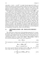
0 5 10 15 20 25 30
10
−6
10
−5

10
−4
10
−3
10
−2
10
−1
10
0
SNR per bit
4-QAM/PSK
64-QAM
64-PSK
16-QAM
16-PSK
BER
FIGURE 1.5 BER comparison between MQAMandMPSKtechniques in the AWGNchannelwith optimumdetection.
to achieve the same bit error rate performance for the MPSK system with smaller M. In other words, we
gain spectral efficiency
2
at the cost of power efficiency
3
with higher-level (M) PSK. For an additive white
Gaussian noise (AWGN) channel, the symbol error rate (SER) P
e
for the MPSK system, using optimum
detection technique, can be approximated [Pro95] for a high signal-to-noise ratio (SNR) as
P
e

= 2Q


2γ
s
sin
π
M

(1.36)
where γ
s
is the SNR per symbol, Q(.) is the Q function, and M is the level of PSK schemes.
2
Spectral efficiency demonstrates the ability of a system (modulation scheme) to accommodate data within an
allocated bandwidth.
3
Power efficiency represents the ability of a system to reliably transmit information at the lowest practical power
level.
Copyright © 2005 by CRC Press LLC
There are many variations in the PSK modulation format that are in use because of better power and
spectral efficiency requirements. Offset QPSK (OQPSK), differential QPSK (DQPSK), and π/4 DQPSK
are a few examples of these PSK modulation formats. In OQPSK, the in-phase and quadrature bit streams
are offset in their relative alignment by one bit period. As a result, the signal trajectories are modified in
such a way that the carrier amplitude does not go through or near zero (the center of the constellation).
In this case the spectral efficiency of a OQPSK-based system remains the same as that in a QPSK-based
system, but the reduced amplitude variations for the former one allow a more power efficient, less linear
radio frequency (RF) power amplifier to be used. For DQPSK modulation, the information is carried
by the transition between states. In some cases there are also restrictions on allowable transitions. For
example, in π/4 DQPSK modulation, the carrier trajectory does not go through the origin [Bur01]. The

π/4 DQPSK modulation format uses two QPSK constellations offset by 45 degrees (π/4 radians). Like
OQPSK, π /4 DQPSK is a power efficient modulation method, and with root cosine filtering it has better
spectral efficiency than Gaussian minimum shift keying (GMSK) [Bur01] modulation.
BPSK and QPSK modulation techniques are used mostly for satellite links because of their simplified
form, reasonable power and spectral efficiencies, and immunity to noise andinterference. Examples include
the Iridium (a voice/data satellite system) and Digital Video Broadcasting Satellite (DVB-S) systems.
Besides, in both IS95 and CDMA2000
4
(also known as 3G IS-2000) cellular systems, BPSK/QPSK and
OQPSK modulation techniques are used in the forward and reverse links, respectively. Eight PSK finds its
application in enhanced data rate for GSM evolution (EDGE) cellular technology. π/4 DQPSK modulation
is used for IS54 [North American Digital Cellular (NADC) system] and cordless personal communications
services in North America, for pacific digital cellular (PDC) services [Rap96] in Japan, and for Trans
European Trunked Radio (TETRA) systems in Europe. In a 3G cellular data-only system (IS856, also
known as cdma2000 1xEV-DO), BPSK modulation is used in the reverse link, while QPSK and eight PSK
modulations along with the quadrature amplitude modulation (QAM) technique (discussed later) are
used in the forward link to support multirate data applications. In the next-generation mobile systems,
researchers are still focusing on different PSK modulations as major modulation techniques. Certainly,
in addition to this, coding and orthogonal frequency division multiplexing (OFDM) techniques are also
considered.
1.3.2.2 Pulse Amplitude Modulation
In this type of digitalmodulation technique themodulating datasignals shift the amplitude of the constant-
phase carrier signal between M number of discrete levels. PAM is also known as amplitude shift keying
(ASK) modulation. The analytical expression for the mth signal waveform in the PAM technique can be
expressed in a general form as
s
m
(t) = A
m
g (t) cos [2π f

c
t +θ], m = 1, 2, , M 0 ≤ t ≤ T (1.37)
where g (t) is the signal pulse shape and A
m
=(2m − 1 + M)d; m =1, 2, , M are the M possible
amplitude levels of the constant-phase (θ) carrier frequency f
c
that convey the transmitted information
for M =2
k
possible k-bit (k being a positive integer) blocks or symbols. The parameter d is related to the
distance between the adjacent signal amplitudes, which is 2d. As in the case of PSK, Gray encoding is also
preferred here for mapping the k information bits into M different amplitudes. The PAM technique finds
its application when it is combined with the PSK modulation technique, as shown later.
1.3.2.3 Quadrature Amplitude Modulation
QAM is simply a combination of the PAM and PSK modulation techniques. In this scheme, two orthogonal
carrier frequencies (in-phase and quadrature carriers), occupying identical frequency bands, are used to
transmit data over a given physical channel. The analytical expression for the mth signal waveform in the
4
/>Copyright © 2005 by CRC Press LLC