How to Display Data- P11 potx
Bạn đang xem bản rút gọn của tài liệu. Xem và tải ngay bản đầy đủ của tài liệu tại đây (145.54 KB, 5 trang )
42 How to Display Data
References
1 Campbell MJ. Time series regression for counts: an investigation into the relation-
ship between Sudden Infant Death Syndrome and environmental temperature.
Journal of the Royal Statistical Society, Series A 1994;157:191–208.
2 Tufte ER. The visual display of quantitative information. Cheshire, Connecticut:
Graphics Press; 1983.
3 Morrell CJ, Walters SJ, Dixon S, Collins K, Brereton LML, Peters J, et al. Cost effec-
tiveness of community leg ulcer clinic: randomised controlled trial. British Medical
Journal 1998;316:1487–91.
4 Freeman JV, Julious S. Describing and summarising data. SCOPE 2005. Vol 14(3).
43
Chapter 5 Displaying the relationship
between two continuous variables
5.1 Introduction
This chapter will concentrate on methods for displaying the relation-ship
between two continuous variables. A large proportion of statisti-cal analy-
ses are conducted to investigate the relationship between two variables for a
particular group of subjects. Such analyses have several purposes:
– To assess whether the two variables are associated (correlation).
– To enable the value of one variable to be predicted from any known value
of the other variable (regression). One variable is regarded as a response
to the other explanatory variable.
– To assess the amount of agreement between the values of the two vari-
ables. Most commonly this situation arises in the comparison of alterna-
tive ways of measuring or assessing the same thing.
– To diagnose of a disease or a condition (present/absent) using the results
of a test with a continuous measurement scale.
The statistical method for assessing the linear association between two con-
tinuous variables is known as correlation. The method for predicting the
value of one continuous variable from another is known as regression. As
correlation and regression are often presented together it is easy to get the
impression that they are inseparable. In fact, they have distinct purposes
and it is relatively rare that one is genuinely interested in performing both
analyses on the same set of data.
However, when preparing to conduct either analysis it is essential to con-
struct a scatter diagram of the values of one of the variables against the
values of the other variable. By drawing a scatter diagram one can see imme-
diately whether or not there is any visual evidence of a straight line or linear
association between the two variables.
5.2 Correlation
Figure 5.1 shows a scatter diagram of the systolic and diastolic blood pres-
sure amongst 96 adults with carotid artery disease aged 42–89 years prior to
44 How to Display Data
220
200
180
160
140
120
100
10090807060 110
Diastolic blood pressure (mmHg)
Systolic blood pressure (mmHg)
Pearson correlation r ϭ 0.62 (P ϭ 0.001)
Figure 5.1 Scatter diagram of systolic vs. diastolic blood pressure for 96 patients with
carotid artery disease.
1
surgery. The data come from a randomised-controlled trial which aimed to
compare outcomes after two forms of surgery (carotid angioplasty (PTA)
and endarterectomy (CEA)) in patients with symptomatic carotid artery
disease.
1
There appears to be some association between the values of the
two variables; we can see that there is a tendency for patients with higher
diastolic blood pressure to have higher systolic blood pressure.
With correlation, it is not important which variable is plotted on the X
(horizontal) axis and which is plotted in the Y (vertical) axis as what is of
interest is to see whether as the values of one variable change, the values of
the other variable change as well. In this example the systolic and diastolic
blood pressure variables could be plotted on either the X or Y-axis. Either
variable could cause or infl uence the other. In contrast, if we were interested
in the relationship between height and weight, then as height to some extent
determines weight and not the other way round (the weight a person is does
not determine their height) it is recommended to plot height on the X-axis
and weight on the Y-axis.
The degree of association, between systolic and diastolic blood pressures in
this example, can be measured using the correlation coeffi cient. The standard
Relationship between two continuous variables 45
method called Pearson’s correlation coeffi cient leads to a quantity called
r which can take any value from Ϫ1 to ϩ1. This measures the degree of
straight line association between the values of the two variables. It is posi-
tive if higher values of one variable are associated with higher values of the
other and negative if one variable tends to be low as the other gets higher.
A correlation of around zero indicates that there is no linear relation between
the values of the two variables. Clearly, the systolic and diastolic blood pres-
sure variables in Figure 5.1 are positively correlated, and the correlation
coeffi cient is r ϭ 0.62. Technical details on how to calculate correlation coef-
fi cients are given in Chapter 9 of Campbell, Machin and Walters.
2
Figure 5.2 shows the same data, but with the origin (systolic blood pres-
sure of 0 mmHg and diastolic blood pressure of 0 mmHg), included for both
the X and Y-axis. In this graph there is a large amount of blank space, since
no patient in this sample has a diastolic blood pressure below 60 mmHg or
a systolic blood pressure below 100 mmHg. This graph clearly shows that
the relationship between systolic and diastolic blood pressure is only valid,
in this sample, for a limited range of diastolic blood pressures between 60
and 110 mmHg. Rather than waste space, the scales on either the horizontal
250
200
150
100
50
0
100806040200 120
Diastolic blood pressure (mmHg)
Systolic blood pressure (mmHg)
Figure 5.2 Scatter diagram of systolic vs. diastolic blood pressure for 96 patients with
carotid artery disease with zero origin for both axes.
1
46 How to Display Data
or vertical axes or both axes can be truncated to refl ect the actual range of
observations for the two variables in the sample. In these circumstances, as
Figure 5.1 illustrates, it is good practice to notch or score the truncated axis
with two parallel line symbols ‘//’ to indicate that the origin or zero value
for the axis has been omitted.
If the sample consisted of different subgroups for whom it was thought
that the correlation might differ then it is possible to use different symbols
and colours for the different subgroups in the scatter diagram. However, if
colour is used, care should be taken as different colours can appear the same
when photocopied. For example, the blood pressure data in Figure 5.1 relates
to 64 men and 32 women. By using different symbols or different colours to
distinguish between men and women it is possible to see visually whether
the relationship between the two blood pressure variables is the same in the
two groups (Figure 5.3). From Figure 5.3, this appears to be the case.
220
200
180
160
140
120
100
10090807060 110
Diastolic blood pressure (mmHg)
Systolic blood pressure (mmHg)
Male (n ϭ 64)
Female (n ϭ 32)
Figure 5.3 Scatter diagram of systolic vs. diastolic blood pressure for 96 patients with
carotid artery disease by sex.
1
Correlation is often used as an exploratory method for investigating the
interrelationships among several continuous variables. Simpson describes a
prospective study in which 98 pre-term infants were given a series of tests
shortly after they were born, in an attempt to predict their outcome after