Introduction to Probability - Chapter 3 ppt

Chapter 3
Combinatorics
3.1 Permutations
Many problems in probability theory require that we count the number of ways
that a particular event can occur. For this, we study the topics of permutations and
combinations. We consider permutations in this section and combinations in the
next section.
Before discussing permutations, it is useful to introduce a general counting tech-
nique that will enable us to solve a variety of counting problems, including the
problem of counting the number of possible permutations of n objects.
Counting Problems
Consider an experiment that takes place in several stages and is such that the
number of outcomes m at the nth stage is independent of the outcomes of the
previous stages. The number m may be different for different stages. We want to
count the number of ways that the entire experiment can be carried out.
Example 3.1 You are eating at
´
Emile’s restaurant and the waiter informs you
that you have (a) two choices for appetizers: soup or juice; (b) three for the main
course: a meat, fish, or vegetable dish; and (c) two for dessert: ice cream or cake.
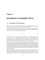
How many possible choices do you have for your complete meal? We illustrate the
possible meals by a tree diagram shown in Figure 3.1. Your menu is decided in three
stages—at each stage the number of possible choices does not depend on what is
chosen in the previous stages: two choices at the first stage, three at the second,
and two at the third. From the tree diagram we see that the total number of choices
is the product of the number of choices at each stage. In this examples we have
2 · 3 · 2 = 12 possible menus. Our menu example is an example of the following
general counting technique. ✷
75

76 CHAPTER 3. COMBINATORICS
ice cream
cake
ice cream
cake
ice cream
cake
ice cream
cake
ice cream
cake
ice cream
cake
(start)
soup
meat
fish
vegetable
juice
meat
fish
vegetable
Figure 3.1: Tree for your menu.
A Counting Technique
A task is to be carried out in a sequence of r stages. There are n
1
ways to carry
out the first stage; for each of these n
1
ways, there are n

2
ways to carry out the
second stage; for each of these n
2
ways, there are n
3
ways to carry out the third
stage, and so forth. Then the total number of ways in which the entire task can be
accomplished is given by the product N = n
1
· n
2
· · n
r
.
Tree Diagrams
It will often be useful to use a tree diagram when studying probabilities of events
relating to experiments that take place in stages and for which we are given the
probabilities for the outcomes at each stage. For example, assume that the owner
of
´
Emile’s restaurant has observed that 80 percent of his customers choose the soup
for an appetizer and 20 percent choose juice. Of those who choose soup, 50 percent
choose meat, 30 percent choose fish, and 20 percent choose the vegetable dish. Of
those who choose juice for an appetizer, 30 percent choose meat, 40 percent choose
fish, and 30 percent choose the vegetable dish. We can use this to estimate the
probabilities at the first two stages as indicated on the tree diagram of Figure 3.2.
We choose for our sample space the set Ω of all possible paths ω = ω
1
, ω

2
,
, ω
6
through the tree. How should we assign our probability distribution? For
example, what probability should we assign to the customer choosing soup and then
the meat? If 8/10 of the customers choose soup and then 1/2 of these choose meat,
a proportion 8/10 · 1/2=4/10 of the customers choose soup and then meat. This
suggests choosing our probability distribution for each path through the tree to be
the product of the probabilities at each of the stages along the path. This results
in the probability measure for the sample points ω indicated in Figure 3.2. (Note
that m(ω
1
)+···+ m(ω
6
) = 1.) From this we see, for example, that the probability

3.1. PERMUTATIONS 77
(start)
soup
meat
fish
vegetable
juice
.8
.2
.2
.3
.3
.4

.5
.3
meat
fish
vegetable
ω
(ω)
ω
ω
ω
ω
ω
ω
.4
.24
.16
.06
.08
.06
m
1
2
3
4
5
6
Figure 3.2: Two-stage probability assignment.
that a customer chooses meat is m(ω
1
)+m(ω

4
)=.46.
We shall say more about these tree measures when we discuss the concept of
conditional probability in Chapter 4. We return now to more counting problems.
Example 3.2 We can show that there are at least two people in Columbus, Ohio,
who have the same three initials. Assuming that each person has three initials,
there are 26 possibilities for a person’s first initial, 26 for the second, and 26 for the
third. Therefore, there are 26
3
=17,576 possible sets of initials. This number is
smaller than the number of people living in Columbus, Ohio; hence, there must be
at least two people with the same three initials. ✷
We consider next the celebrated birthday problem—often used to show that
naive intuition cannot always be trusted in probability.
Birthday Problem
Example 3.3 How many people do we need to have in a room to make it a favorable
bet (probability of success greater than 1/2) that two people in the room will have
the same birthday?
Since there are 365 possible birthdays, it is tempting to guess that we would
need about 1/2 this number, or 183. You would surely win this bet. In fact, the
number required for a favorable bet is only 23. To show this, we find the probability
p
r
that, in a room with r people, there is no duplication of birthdays; we will have
a favorable bet if this probability is less than one half.

78 CHAPTER 3. COMBINATORICS
Number of people Probability that all birthdays are different
20 .5885616
21 .5563117

22 .5243047
23 .4927028
24 .4616557
25 .4313003
Table 3.1: Birthday problem.
Assume that there are 365 possible birthdays for each person (we ignore leap
years). Order the people from 1 to r. For a sample point ω, we choose a possible
sequence of length r of birthdays each chosen as one of the 365 possible dates.
There are 365 possibilities for the first element of the sequence, and for each of
these choices there are 365 for the second, and so forth, making 365
r
possible
sequences of birthdays. We must find the number of these sequences that have no
duplication of birthdays. For such a sequence, we can choose any of the 365 days
for the first element, then any of the remaining 364 for the second, 363 for the third,
and so forth, until we make r choices. For the rth choice, there will be 365 −r +1
possibilities. Hence, the total number of sequences with no duplications is
365 ·364 · 363 · · (365 −r +1).
Thus, assuming that each sequence is equally likely,
p
r
=
365 ·364 · · (365 − r +1)
365
r
.
We denote the product
(n)(n −1) ···(n −r +1)
by (n)
r

(read “n down r,” or “n lower r”). Thus,
p
r
=
(365)
r
(365)
r
.
The program Birthday carries out this computation and prints the probabilities
for r = 20 to 25. Running this program, we get the results shown in Table 3.1. As
we asserted above, the probability for no duplication changes from greater than one
half to less than one half as we move from 22 to 23 people. To see how unlikely it is
that we would lose our bet for larger numbers of people, we have run the program
again, printing out values from r =10tor = 100 in steps of 10. We see that in
a room of 40 people the odds already heavily favor a duplication, and in a room
of 100 the odds are overwhelmingly in favor of a duplication. We have assumed
that birthdays are equally likely to fall on any particular day. Statistical evidence
suggests that this is not true. However, it is intuitively clear (but not easy to prove)
that this makes it even more likely to have a duplication with a group of 23 people.
(See Exercise 19 to find out what happens on planets with more or fewer than 365
days per year.) ✷

3.1. PERMUTATIONS 79
Number of people Probability that all birthdays are different
10 .8830518
20 .5885616
30 .2936838
40 .1087682
50 .0296264

60 .0058773
70 .0008404
80 .0000857
90 .0000062
100 .0000003
Table 3.2: Birthday problem.
We now turn to the topic of permutations.
Permutations
Definition 3.1 Let A be any finite set. A permutation of A is a one-to-one mapping
of A onto itself. ✷
To specify a particular permutation we list the elements of A and, under them,
show where each element is sent by the one-to-one mapping. For example, if A =
{a, b, c} a possible permutation σ would be
σ =

abc
bca

.
By the permutation σ, a is sent to b, b is sent to c, and c is sent to a. The
condition that the mapping be one-to-one means that no two elements of A are
sent, by the mapping, into the same element of A.
We can put the elements of our set in some order and rename them 1, 2, , n.
Then, a typical permutation of the set A = {a
1
,a
2
,a
3
,a

4
} can be written in the
form
σ =

1234
2143

,
indicating that a
1
went to a
2
, a
2
to a
1
, a
3
to a
4
, and a
4
to a
3
.
Ifwealwayschoosethetoprowtobe1234then, to prescribe the permutation,
we need only give the bottom row, with the understanding that this tells us where 1
goes, 2 goes, and so forth, under the mapping. When this is done, the permutation
is often called a rearrangement of the n objects 1, 2, 3, , n. For example, all

possible permutations, or rearrangements, of the numbers A = {1, 2, 3} are:
123, 132, 213, 231, 312, 321 .
It is an easy matter to count the number of possible permutations of n objects.
By our general counting principle, there are n ways to assign the first element, for

80 CHAPTER 3. COMBINATORICS
nn!
01
11
22
36
424
5 120
6 720
7 5040
8 40320
9 362880
10 3628800
Table 3.3: Values of the factorial function.
each of these we have n − 1 ways to assign the second object, n − 2 for the third,
and so forth. This proves the following theorem.
Theorem 3.1 The total number of permutations of a set A of n elements is given
by n ·(n − 1) ·(n − 2) · · 1. ✷
It is sometimes helpful to consider orderings of subsets of a given set. This
prompts the following definition.
Definition 3.2 Let A be an n-element set, and let k be an integer between 0 and
n. Then a k-permutation of A is an ordered listing of a subset of A of size k. ✷
Using the same techniques as in the last theorem, the following result is easily
proved.
Theorem 3.2 The total number of k-permutations of a set A of n elements is given

by n ·(n − 1) · (n −2) · · (n − k + 1). ✷
Factorials
The number given in Theorem 3.1 is called n factorial, and is denoted by n!. The
expression 0! is defined to be 1 to make certain formulas come out simpler. The
first few values of this function are shown in Table 3.3. The reader will note that
this function grows very rapidly.
The expression n! will enter into many of our calculations, and we shall need to
have some estimate of its magnitude when n is large. It is clearly not practical to
make exact calculations in this case. We shall instead use a result called Stirling’s
formula. Before stating this formula we need a definition.

3.1. PERMUTATIONS 81
nn! Approximation Ratio
1 1 .922 1.084
2 2 1.919 1.042
3 6 5.836 1.028
4 24 23.506 1.021
5 120 118.019 1.016
6 720 710.078 1.013
7 5040 4980.396 1.011
8 40320 39902.395 1.010
9 362880 359536.873 1.009
10 3628800 3598696.619 1.008
Table 3.4: Stirling approximations to the factorial function.
Definition 3.3 Let a
n
and b
n
be two sequences of numbers. We say that a
n

is
asymptotically equal to b
n
, and write a
n
∼ b
n
,if
lim
n→∞
a
n
b
n
=1.
✷
Example 3.4 If a
n
= n +
√
n and b
n
= n then, since a
n
/b
n
=1+1/
√
n and this
ratio tends to 1 as n tends to infinity, we have a

n
∼ b
n
. ✷
Theorem 3.3 (Stirling’s Formula) The sequence n! is asymptotically equal to
n
n
e
−n
√
2πn .
✷
The proof of Stirling’s formula may be found in most analysis texts. Let us
verify this approximation by using the computer. The program StirlingApprox-
imations prints n!, the Stirling approximation, and, finally, the ratio of these two
numbers. Sample output of this program is shown in Table 3.4. Note that, while
the ratio of the numbers is getting closer to 1, the difference between the exact
value and the approximation is increasing, and indeed, this difference will tend to
infinity as n tends to infinity, even though the ratio tends to 1. (This was also true
in our Example 3.4 where n +
√
n ∼ n, but the difference is
√
n.)
Generating Random Permutations
We now consider the question of generating a random permutation of the integers
between 1 and n. Consider the following experiment. We start with a deck of n
cards, labelled 1 through n. We choose a random card out of the deck, note its label,
and put the card aside. We repeat this process until all n cards have been chosen.
It is clear that each permutation of the integers from 1 to n can occur as a sequence

82 CHAPTER 3. COMBINATORICS
Number of fixed points Fraction of permutations
n=10 n=20 n=30
0 .362 .370 .358
1 .368 .396 .358
2 .202 .164 .192
3 .052 .060 .070
4 .012 .008 .020
5 .004 .002 .002
Average number of fixed points .996 .948 1.042
Table 3.5: Fixed point distributions.
of labels in this experiment, and that each sequence of labels is equally likely to
occur. In our implementations of the computer algorithms, the above procedure is
called RandomPermutation.
Fixed Points
There are many interesting problems that relate to properties of a permutation
chosen at random from the set of all permutations of a given finite set. For example,
since a permutation is a one-to-one mapping of the set onto itself, it is interesting to
ask how many points are mapped onto themselves. We call such points fixed points
of the mapping.
Let p
k
(n) be the probability that a random permutation of the set {1, 2, ,n}
has exactly k fixed points. We will attempt to learn something about these prob-
abilities using simulation. The program FixedPoints uses the procedure Ran-
domPermutation to generate random permutations and count fixed points. The
program prints the proportion of times that there are k fixed points as well as the
average number of fixed points. The results of this program for 500 simulations for
the cases n = 10, 20, and 30 are shown in Table 3.5. Notice the rather surprising

fact that our estimates for the probabilities do not seem to depend very heavily on
the number of elements in the permutation. For example, the probability that there
are no fixed points, when n =10, 20, or 30 is estimated to be between .35 and .37.
We shall see later (see Example 3.12) that for n ≥ 10 the exact probabilities p
n
(0)
are, to six decimal place accuracy, equal to 1/e ≈ .367879. Thus, for all practi-
cal purposes, after n = 10 the probability that a random permutation of the set
{1, 2, ,n} does not depend upon n. These simulations also suggest that the av-
erage number of fixed points is close to 1. It can be shown (see Example 6.8) that
the average is exactly equal to 1 for all n.
More picturesque versions of the fixed-point problem are: You have arranged
the books on your book shelf in alphabetical order by author and they get returned
to your shelf at random; what is the probability that exactly k of the books end up
in their correct position? (The library problem.) In a restaurant n hats are checked
and they are hopelessly scrambled; what is the probability that no one gets his own
hat back? (The hat check problem.) In the Historical Remarks at the end of this
section, we give one method for solving the hat check problem exactly. Another

3.1. PERMUTATIONS 83
Date Snowfall in inches
1974 75
1975 88
1976 72
1977 110
1978 85
1979 30
1980 55
1981 86
1982 51

1983 64
Table 3.6: Snowfall in Hanover.
Year 123 45678910
Ranking 6951071382 4
Table 3.7: Ranking of total snowfall.
method is given in Example 3.12.
Records
Here is another interesting probability problem that involves permutations. Esti-
mates for the amount of measured snow in inches in Hanover, New Hampshire, in
the ten years from 1974 to 1983 are shown in Table 3.6. Suppose we have started
keeping records in 1974. Then our first year’s snowfall could be considered a record
snowfall starting from this year. A new record was established in 1975; the next
record was established in 1977, and there were no new records established after
this year. Thus, in this ten-year period, there were three records established: 1974,
1975, and 1977. The question that we ask is: How many records should we expect
to be established in such a ten-year period? We can count the number of records
in terms of a permutation as follows: We number the years from 1 to 10. The
actual amounts of snowfall are not important but their relative sizes are. We can,
therefore, change the numbers measuring snowfalls to numbers 1 to 10 by replacing
the smallest number by 1, the next smallest by 2, and so forth. (We assume that
there are no ties.) For our example, we obtain the data shown in Table 3.7.
This gives us a permutation of the numbers from 1 to 10 and, from this per-
mutation, we can read off the records; they are in years 1, 2, and 4. Thus we can
define records for a permutation as follows:
Definition 3.4 Let σ be a permutation of the set {1, 2, ,n}. Then i is a record
of σ if either i =1orσ(j) <σ(i) for every j =1, , i− 1. ✷
Now if we regard all rankings of snowfalls over an n-year period to be equally
likely (and allow no ties), we can estimate the probability that there will be k
records in n years as well as the average number of records by simulation.

84 CHAPTER 3. COMBINATORICS
We have written a program Records that counts the number of records in ran-
domly chosen permutations. We have run this program for the cases n = 10, 20, 30.
For n = 10 the average number of records is 2.968, for 20 it is 3.656, and for 30
it is 3.960. We see now that the averages increase, but very slowly. We shall see
later (see Example 6.11) that the average number is approximately log n. Since
log 10 = 2.3, log 20 = 3, and log 30 = 3.4, this is consistent with the results of our
simulations.
As remarked earlier, we shall be able to obtain formulas for exact results of
certain problems of the above type. However, only minor changes in the problem
make this impossible. The power of simulation is that minor changes in a problem
do not make the simulation much more difficult. (See Exercise 20 for an interesting
variation of the hat check problem.)
List of Permutations
Another method to solve problems that is not sensitive to small changes in the
problem is to have the computer simply list all possible permutations and count the
fraction that have the desired property. The program AllPermutations produces
a list of all of the permutations of n. When we try running this program, we run
into a limitation on the use of the computer. The number of permutations of n
increases so rapidly that even to list all permutations of 20 objects is impractical.
Historical Remarks
Our basic counting principle stated that if you can do one thing in r ways and for
each of these another thing in s ways, then you can do the pair in rs ways. This
is such a self-evident result that you might expect that it occurred very early in
mathematics. N. L. Biggs suggests that we might trace an example of this principle
as follows: First, he relates a popular nursery rhyme dating back to at least 1730:
As I was going to St. Ives,
I met a man with seven wives,
Each wife had seven sacks,
Each sack had seven cats,

Each cat had seven kits.
Kits, cats, sacks and wives,
How many were going to St. Ives?
(You need our principle only if you are not clever enough to realize that you are
supposed to answer one, since only the narrator is going to St. Ives; the others are
going in the other direction!)
He also gives a problem appearing on one of the oldest surviving mathematical
manuscripts of about 1650
B.C., roughly translated as:

3.1. PERMUTATIONS 85
Houses 7
Cats 49
Mice 343
Wheat 2401
Hekat 16807
19607
The following interpretation has been suggested: there are seven houses, each
with seven cats; each cat kills seven mice; each mouse would have eaten seven heads
of wheat, each of which would have produced seven hekat measures of grain. With
this interpretation, the table answers the question of how many hekat measures
were saved by the cats’ actions. It is not clear why the writer of the table wanted
to add the numbers together.
1
One of the earliest uses of factorials occurred in Euclid’s proof that there are
infinitely many prime numbers. Euclid argued that there must be a prime number
between n and n! + 1 as follows: n! and n! + 1 cannot have common factors. Either
n! +1 is prime or it has a proper factor. In the latter case, this factor cannot divide
n! and hence must be between n and n! + 1. If this factor is not prime, then it
has a factor that, by the same argument, must be bigger than n. In this way, we

eventually reach a prime bigger than n, and this holds for all n.
The “n!” rule for the number of permutations seems to have occurred first in
India. Examples have been found as early as 300
B.C., and by the eleventh century
the general formula seems to have been well known in India and then in the Arab
countries.
The hat check problem is found in an early probability book written by de Mont-
mort and first printed in 1708.
2
It appears in the form of a game called Treize. In
a simplified version of this game considered by de Montmort one turns over cards
numbered 1 to 13, calling out 1, 2, , 13asthe cards are examined. De Montmort
asked for the probability that no card that is turned up agrees with the number
called out.
This probability is the same as the probability that a random permutation of
13 elements has no fixed point. De Montmort solved this problem by the use of a
recursion relation as follows: let w
n
be the number of permutations of n elements
with no fixed point (such permutations are called derangements). Then w
1
= 0 and
w
2
=1.
Now assume that n ≥ 3 and choose a derangement of the integers between 1 and
n. Let k be the integer in the first position in this derangement. By the definition of
derangement, we have k = 1. There are two possibilities of interest concerning the
position of 1 in the derangement: either 1 is in the kth position or it is elsewhere. In
the first case, the n −2 remaining integers can be positioned in w

n−2
ways without
resulting in any fixed points. In the second case, we consider the set of integers
{1, 2, ,k− 1,k +1, ,n}. The numbers in this set must occupy the positions
{2, 3, ,n} so that none of the numbers other than 1 in this set are fixed, and
1
N. L. Biggs, “The Roots of Combinatorics,” Historia Mathematica, vol. 6 (1979), pp. 109–136.
2
P. R. de Montmort, Essay d’Analyse sur des Jeux de Hazard, 2d ed. (Paris: Quillau, 1713).

86 CHAPTER 3. COMBINATORICS
also so that 1 is not in position k. The number of ways of achieving this kind of
arrangement is just w
n−1
. Since there are n − 1 possible values of k, we see that
w
n
=(n − 1)w
n−1
+(n − 1)w
n−2
for n ≥ 3. One might conjecture from this last equation that the sequence {w
n
}
grows like the sequence {n!}.
In fact, it is easy to prove by induction that
w
n
= nw
n−1

+(−1)
n
.
Then p
i
= w
i
/i! satisfies
p
i
− p
i−1
=
(−1)
i
i!
.
If we sum from i =2ton, and use the fact that p
1
= 0, we obtain
p
n
=
1
2!
−
1
3!
+ ···+
(−1)

n
n!
.
This agrees with the first n + 1 terms of the expansion for e
x
for x = −1 and hence
for large n is approximately e
−1
≈ .368. David remarks that this was possibly
the first use of the exponential function in probability.
3
We shall see another way
to derive de Montmort’s result in the next section, using a method known as the
Inclusion-Exclusion method.
Recently, a related problem appeared in a column of Marilyn vos Savant.
4
Charles Price wrote to ask about his experience playing a certain form of solitaire,
sometimes called “frustration solitaire.” In this particular game, a deck of cards
is shuffled, and then dealt out, one card at a time. As the cards are being dealt,
the player counts from 1 to 13, and then starts again at 1. (Thus, each number is
counted four times.) If a number that is being counted coincides with the rank of
the card that is being turned up, then the player loses the game. Price found that
he he rarely won and wondered how often he should win. Vos Savant remarked that
the expected number of matches is 4 so it should be difficult to win the game.
Finding the chance of winning is a harder problem than the one that de Mont-
mort solved because, when one goes through the entire deck, there are different
patterns for the matches that might occur. For example matches may occur for two
cards of the same rank, say two aces, or for two different ranks, say a two and a
three.
A discussion of this problem can be found in Riordan.

5
In this book, it is shown
that as n →∞, the probability of no matches tends to 1/e
4
.
The original game of Treize is more difficult to analyze than frustration solitaire.
The game of Treize is played as follows. One person is chosen as dealer and the
others are players. Each player, other than the dealer, puts up a stake. The dealer
shuffles the cards and turns them up one at a time calling out, “Ace, two, three, ,
3
F. N. David, Games, Gods and Gambling (London: Griffin, 1962), p. 146.
4
M. vos Savant, Ask Marilyn, Parade Magazine, Boston Globe, 21 August 1994.
5
J. Riordan, An Introduction to Combinatorial Analysis, (New York: John Wiley & Sons,
1958).

3.1. PERMUTATIONS 87
king,” just as in frustration solitaire. If the dealer goes through the 13 cards without
a match he pays the players an amount equal to their stake, and the deal passes to
someone else. If there is a match the dealer collects the players’ stakes; the players
put up new stakes, and the dealer continues through the deck, calling out, “Ace,
two, three, ” If the dealer runs out of cards he reshuffles and continues the count
where he left off. He continues until there is a run of 13 without a match and then
a new dealer is chosen.
The question at this point is how much money can the dealer expect to win from
each player. De Montmort found that if each player puts up a stake of 1, say, then
the dealer will win approximately .801 from each player.
Peter Doyle calculated the exact amount that the dealer can expect to win. The
answer is:

26516072156010218582227607912734182784642120482136091446715371962089931
52311343541724554334912870541440299239251607694113500080775917818512013
82176876653563173852874555859367254632009477403727395572807459384342747
87664965076063990538261189388143513547366316017004945507201764278828306
60117107953633142734382477922709835281753299035988581413688367655833113
24476153310720627474169719301806649152698704084383914217907906954976036
28528211590140316202120601549126920880824913325553882692055427830810368
57818861208758248800680978640438118582834877542560955550662878927123048
26997601700116233592793308297533642193505074540268925683193887821301442
70519791882/
33036929133582592220117220713156071114975101149831063364072138969878007
99647204708825303387525892236581323015628005621143427290625658974433971
65719454122908007086289841306087561302818991167357863623756067184986491
35353553622197448890223267101158801016285931351979294387223277033396967
79797069933475802423676949873661605184031477561560393380257070970711959
69641268242455013319879747054693517809383750593488858698672364846950539
88868628582609905586271001318150621134407056983214740221851567706672080
94586589378459432799868706334161812988630496327287254818458879353024498
00322425586446741048147720934108061350613503856973048971213063937040515
59533731591.
This is .803 to 3 decimal places. A description of the algorithm used to find this
answer can be found on his Web page.
6
A discussion of this problem and other
problems can be found in Doyle et al.
7
The birthday problem does not seem to have a very old history. Problems of
this type were first discussed by von Mises.
8
It was made popular in the 1950s by

Feller’s book.
9
6
P. Doyle, “Solution to Montmort’s Probleme du Treize,” />7
P. Doyle, C. Grinstead, and J. Snell, “Frustration Solitaire,” UMAP Journal, vol. 16, no. 2
(1995), pp. 137-145.
8
R. von Mises, “
¨
Uber Aufteilungs- und Besetzungs-Wahrscheinlichkeiten,” Revue de la Facult´e
des Sciences de l’Universit´e d’Istanbul, N. S. vol. 4 (1938-39), pp. 145-163.
9
W. Feller, Introduction to Probability Theory and Its Applications, vol. 1, 3rd ed. (New York:

88 CHAPTER 3. COMBINATORICS
Stirling presented his formula
n! ∼
√
2πn

n
e

n
in his work Methodus Differentialis published in 1730.
10
This approximation was
used by de Moivre in establishing his celebrated central limit theorem that we
will study in Chapter 9. De Moivre himself had independently established this
approximation, but without identifying the constant π. Having established the

approximation
2B
√
n
for the central term of the binomial distribution, where the constant B was deter-
mined by an infinite series, de Moivre writes:
. . . my worthy and learned Friend, Mr. James Stirling, who had applied
himself after me to that inquiry, found that the Quantity B did denote
the Square-root of the Circumference of a Circle whose Radius is Unity,
so that if that Circumference be called c the Ratio of the middle Term
to the Sum of all Terms will be expressed by 2/
√
nc
11
Exercises
1 Four people are to be arranged in a row to have their picture taken. In how
many ways can this be done?
2 An automobile manufacturer has four colors available for automobile exteri-
ors and three for interiors. How many different color combinations can he
produce?
3 In a digital computer, a bit is one of the integers {0,1}, and a word is any
string of 32 bits. How many different words are possible?
4 What is the probability that at least 2 of the presidents of the United States
have died on the same day of the year? If you bet this has happened, would
you win your bet?
5 There are three different routes connecting city A to city B. How many ways
can a round trip be made from A to B and back? How many ways if it is
desired to take a different route on the way back?
6 In arranging people around a circular table, we take into account their seats
relative to each other, not the actual position of any one person. Show that

n people can be arranged around a circular table in (n − 1)! ways.
John Wiley & Sons, 1968).
10
J. Stirling, Methodus Differentialis, (London: Bowyer, 1730).
11
A. de Moivre, The Doctrine of Chances, 3rd ed. (London: Millar, 1756).

3.1. PERMUTATIONS 89
7 Five people get on an elevator that stops at five floors. Assuming that each
has an equal probability of going to any one floor, find the probability that
they all get off at different floors.
8 A finite set Ω has n elements. Show that if we count the empty set and Ω as
subsets, there are 2
n
subsets of Ω.
9 A more refined inequality for approximating n! is given by
√
2πn

n
e

n
e
1/(12n+1)
<n! <
√
2πn

n

e

n
e
1/(12n)
.
Write a computer program to illustrate this inequality for n = 1 to 9.
10 A deck of ordinary cards is shuffled and 13 cards are dealt. What is the
probability that the last card dealt is an ace?
11 There are n applicants for the director of computing. The applicants are inter-
viewed independently by each member of the three-person search committee
and ranked from 1 to n. A candidate will be hired if he or she is ranked first
by at least two of the three interviewers. Find the probability that a candidate
will be accepted if the members of the committee really have no ability at all
to judge the candidates and just rank the candidates randomly. In particular,
compare this probability for the case of three candidates and the case of ten
candidates.
12 A symphony orchestra has in its repertoire 30 Haydn symphonies, 15 modern
works, and 9 Beethoven symphonies. Its program always consists of a Haydn
symphony followed by a modern work, and then a Beethoven symphony.
(a) How many different programs can it play?
(b) How many different programs are there if the three pieces can be played
in any order?
(c) How many different three-piece programs are there if more than one
piece from the same category can be played and they can be played in
any order?
13 A certain state has license plates showing three numbers and three letters.
How many different license plates are possible
(a) if the numbers must come before the letters?
(b) if there is no restriction on where the letters and numbers appear?

14 The door on the computer center has a lock which has five buttons numbered
from 1 to 5. The combination of numbers that opens the lock is a sequence
of five numbers and is reset every week.
(a) How many combinations are possible if every button must be used once?

90 CHAPTER 3. COMBINATORICS
(b) Assume that the lock can also have combinations that require you to
push two buttons simultaneously and then the other three one at a time.
How many more combinations does this permit?
15 A computing center has 3 processors that receive n jobs, with the jobs assigned
to the processors purely at random so that all of the 3
n
possible assignments
are equally likely. Find the probability that exactly one processor has no jobs.
16 Prove that at least two people in Atlanta, Georgia, have the same initials,
assuming no one has more than four initials.
17 Find a formula for the probability that among a set of n people, at least two
have their birthdays in the same month of the year (assuming the months are
equally likely for birthdays).
18 Consider the problem of finding the probability of more than one coincidence
of birthdays in a group of n people. These include, for example, three people
with the same birthday, or two pairs of people with the same birthday, or
larger coincidences. Show how you could compute this probability, and write
a computer program to carry out this computation. Use your program to find
the smallest number of people for which it would be a favorable bet that there
would be more than one coincidence of birthdays.
*19 Suppose that on planet Zorg a year has n days, and that the lifeforms there
are equally likely to have hatched on any day of the year. We would like
to estimate d, which is the minimum number of lifeforms needed so that the
probability of at least two sharing a birthday exceeds 1/2.

(a) In Example 3.3, it was shown that in a set of d lifeforms, the probability
that no two life forms share a birthday is
(n)
d
n
d
,
where (n)
d
=(n)(n − 1) ···(n − d + 1). Thus, we would like to set this
equal to 1/2 and solve for d.
(b) Using Stirling’s Formula, show that
(n)
d
n
d
∼

1+
d
n −d

n−d+1/2
e
−d
.
(c) Now take the logarithm of the right-hand expression, and use the fact
that for small values of x,wehave
log(1 + x) ∼ x −
x

2
2
.
(We are implicitly using the fact that d is of smaller order of magnitude
than n. We will also use this fact in part (d).)

3.1. PERMUTATIONS 91
(d) Set the expression found in part (c) equal to −log(2), and solve for d as
a function of n, thereby showing that
d ∼

2(log 2) n.
Hint: If all three summands in the expression found in part (b) are used,
one obtains a cubic equation in d. If the smallest of the three terms is
thrown away, one obtains a quadratic equation in d.
(e) Use a computer to calculate the exact values of d for various values of
n. Compare these values with the approximate values obtained by using
the answer to part d).
20 At a mathematical conference, ten participants are randomly seated around
a circular table for meals. Using simulation, estimate the probability that no
two people sit next to each other at both lunch and dinner. Can you make an
intelligent conjecture for the case of n participants when n is large?
21 Modify the program AllPermutations to count the number of permutations
of n objects that have exactly j fixed points for j = 0, 1, 2, , n. Run
your program for n = 2 to 6. Make a conjecture for the relation between the
number that have 0 fixed points and the number that have exactly 1 fixed
point. A proof of the correct conjecture can be found in Wilf.
12
22 Mr. Wimply Dimple, one of London’s most prestigious watch makers, has
come to Sherlock Holmes in a panic, having discovered that someone has

been producing and selling crude counterfeits of his best selling watch. The 16
counterfeits so far discovered bear stamped numbers, all of which fall between
1 and 56, and Dimple is anxious to know the extent of the forger’s work. All
present agree that it seems reasonable to assume that the counterfeits thus
far produced bear consecutive numbers from 1 to whatever the total number
is.
“Chin up, Dimple,” opines Dr. Watson. “I shouldn’t worry overly much if
I were you; the Maximum Likelihood Principle, which estimates the total
number as precisely that which gives the highest probability for the series
of numbers found, suggests that we guess 56 itself as the total. Thus, your
forgers are not a big operation, and we shall have them safely behind bars
before your business suffers significantly.”
“Stuff, nonsense, and bother your fancy principles, Watson,” counters Holmes.
“Anyone can see that, of course, there must be quite a few more than 56
watches—why the odds of our having discovered precisely the highest num-
bered watch made are laughably negligible. A much better guess would be
twice 56.”
(a) Show that Watson is correct that the Maximum Likelihood Principle
gives 56.
12
H. S. Wilf, “A Bijection in the Theory of Derangements,” Mathematics Magazine, vol. 57,
no. 1 (1984), pp. 37–40.

92 CHAPTER 3. COMBINATORICS
(b) Write a computer program to compare Holmes’s and Watson’s guessing
strategies as follows: fix a total N and choose 16 integers randomly
between 1 and N . Let m denote the largest of these. Then Watson’s
guess for N is m, while Holmes’s is 2m. See which of these is closer to
N. Repeat this experiment (with N still fixed) a hundred or more times,
and determine the proportion of times that each comes closer. Whose

seems to be the better strategy?
23 Barbara Smith is interviewing candidates to be her secretary. As she inter-
views the candidates, she can determine the relative rank of the candidates
but not the true rank. Thus, if there are six candidates and their true rank is
6, 1, 4, 2, 3, 5, (where 1 is best) then after she had interviewed the first three
candidates she would rank them 3, 1, 2. As she interviews each candidate,
she must either accept or reject the candidate. If she does not accept the
candidate after the interview, the candidate is lost to her. She wants to de-
cide on a strategy for deciding when to stop and accept a candidate that will
maximize the probability of getting the best candidate. Assume that there
are n candidates and they arrive in a random rank order.
(a) What is the probability that Barbara gets the best candidate if she inter-
views all of the candidates? What is it if she chooses the first candidate?
(b) Assume that Barbara decides to interview the first half of the candidates
and then continue interviewing until getting a candidate better than any
candidate seen so far. Show that she has a better than 25 percent chance
of ending up with the best candidate.
24 For the task described in Exercise 23, it can be shown
13
that the best strategy
is to pass over the first k − 1 candidates where k is the smallest integer for
which
1
k
+
1
k +1
+ ···+
1
n −1

≤ 1 .
Using this strategy the probability of getting the best candidate is approxi-
mately 1/e = .368. Write a program to simulate Barbara Smith’s interviewing
if she uses this optimal strategy, using n = 10, and see if you can verify that
the probability of success is approximately 1/e.
3.2 Combinations
Having mastered permutations, we now consider combinations. Let U be a set with
n elements; we want to count the number of distinct subsets of the set U that have
exactly j elements. The empty set and the set U are considered to be subsets of U .
The empty set is usually denoted by φ.
13
E. B. Dynkin and A. A. Yushkevich, Markov Processes: Theorems and Problems, trans. J. S.
Wood (New York: Plenum, 1969).

3.2. COMBINATIONS 93
Example 3.5 Let U = {a, b, c}. The subsets of U are
φ, {a}, {b}, {c}, {a, b}, {a, c}, {b, c}, {a, b, c} .
✷
Binomial Coefficients
The number of distinct subsets with j elements that can be chosen from a set with
n elements is denoted by

n
j

, and is pronounced “n choose j.” The number

n
j


is
called a binomial coefficient. This terminology comes from an application to algebra
which will be discussed later in this section.
In the above example, there is one subset with no elements, three subsets with
exactly 1 element, three subsets with exactly 2 elements, and one subset with exactly
3 elements. Thus,

3
0

=1,

3
1

=3,

3
2

= 3, and

3
3

= 1. Note that there are
2
3
= 8 subsets in all. (We have already seen that a set with n elements has 2
n

subsets; see Exercise 3.1.8.) It follows that

3
0

+

3
1

+

3
2

+

3
3

=2
3
=8,

n
0

=

n

n

=1.
Assume that n>0. Then, since there is only one way to choose a set with no
elements and only one way to choose a set with n elements, the remaining values
of

n
j

are determined by the following recurrence relation:
Theorem 3.4 For integers n and j, with 0 <j<n, the binomial coefficients
satisfy:

n
j

=

n −1
j

+

n −1
j −1

. (3.1)
Proof. We wish to choose a subset of j elements. Choose an element u of U .
Assume first that we do not want u in the subset. Then we must choose the j

elements from a set of n −1 elements; this can be done in

n−1
j

ways. On the other
hand, assume that we do want u in the subset. Then we must choose the other
j − 1 elements from the remaining n − 1 elements of U ; this can be done in

n−1
j−1

ways. Since u is either in our subset or not, the number of ways that we can choose
a subset of j elements is the sum of the number of subsets of j elements which have
u as a member and the number which do not—this is what Equation 3.1 states. ✷
The binomial coefficient

n
j

is defined to be 0, if j<0orifj>n. With this
definition, the restrictions on j in Theorem 3.4 are unnecessary.

94 CHAPTER 3. COMBINATORICS
n = 0 1
10 1 10 45 120 210 252 210 120 45 10 1
9 1 9 36 84 126 126 84 36 9 1
8 1 8 28 56 70 56 28 8 1
7 1 7 21 35 35 21 7 1
6 1 6 15 20 15 6 1

5 1 5 10 10 5 1
4 1 4 6 4 1
3 1 3 3 1
2 1 2 1
1 1 1
j = 0 1 2 3 4 5 6 7 8 9 10
Figure 3.3: Pascal’s triangle.
Pascal’s Triangle
The relation 3.1, together with the knowledge that

n
0

=

n
n

=1,
determines completely the numbers

n
j

. We can use these relations to determine
the famous triangle of Pascal, which exhibits all these numbers in matrix form (see
Figure 3.3).
The nth row of this triangle has the entries

n

0

,

n
1

, ,

n
n

. We know that the
first and last of these numbers are 1. The remaining numbers are determined by
the recurrence relation Equation 3.1; that is, the entry

n
j

for 0 <j<nin the
nth row of Pascal’s triangle is the sum of the entry immediately above and the one
immediately to its left in the (n −1)st row. For example,

5
2

=6+4=10.
This algorithm for constructing Pascal’s triangle can be used to write a computer
program to compute the binomial coefficients. You are asked to do this in Exercise 4.
While Pascal’s triangle provides a way to construct recursively the binomial

coefficients, it is also possible to give a formula for

n
j

.
Theorem 3.5 The binomial coefficients are given by the formula

n
j

=
(n)
j
j!
. (3.2)
Proof. Each subset of size j of a set of size n can be ordered in j! ways. Each of
these orderings is a j-permutation of the set of size n. The number of j-permutations
is (n)
j
, so the number of subsets of size j is
(n)
j
j!
.
This completes the proof. ✷

3.2. COMBINATIONS 95
The above formula can be rewritten in the form


n
j

=
n!
j!(n − j)!
.
This immediately shows that

n
j

=

n
n −j

.
When using Equation 3.2 in the calculation of

n
j

, if one alternates the multi-
plications and divisions, then all of the intermediate values in the calculation are
integers. Furthermore, none of these intermediate values exceed the final value.
(See Exercise 40.)
Another point that should be made concerning Equation 3.2 is that if it is used
to define the binomial coefficients, then it is no longer necessary to require n to be
a positive integer. The variable j must still be a non-negative integer under this

definition. This idea is useful when extending the Binomial Theorem to general
exponents. (The Binomial Theorem for non-negative integer exponents is given
below as Theorem 3.7.)
Poker Hands
Example 3.6 Poker players sometimes wonder why a four of a kind beats a full
house. A poker hand is a random subset of 5 elements from a deck of 52 cards.
A hand has four of a kind if it has four cards with the same value—for example,
four sixes or four kings. It is a full house if it has three of one value and two of a
second—for example, three twos and two queens. Let us see which hand is more
likely. How many hands have four of a kind? There are 13 ways that we can specify
the value for the four cards. For each of these, there are 48 possibilities for the fifth
card. Thus, the number of four-of-a-kind hands is 13 · 48 = 624. Since the total
number of possible hands is

52
5

= 2598960, the probability of a hand with four of
a kind is 624/2598960 = .00024.
Now consider the case of a full house; how many such hands are there? There
are 13 choices for the value which occurs three times; for each of these there are

4
3

= 4 choices for the particular three cards of this value that are in the hand.
Having picked these three cards, there are 12 possibilities for the value which occurs
twice; for each of these there are

4

2

= 6 possibilities for the particular pair of this
value. Thus, the number of full houses is 13 · 4 · 12 ·6 = 3744, and the probability
of obtaining a hand with a full house is 3744/2598960 = .0014. Thus, while both
types of hands are unlikely, you are six times more likely to obtain a full house than
four of a kind. ✷

96 CHAPTER 3. COMBINATORICS
(start)
S
F
F
F
F
S
S
S
S
S
S
F
F
F
p
q
p
p
q
p q

q p
q p
q
q
q
q
q
q
p
p
p
p
p
p
q
q
p
p
q
m (ω)
ω
ω
ω
ω
ω
ω
ω
ω
ω

2
3
3
2
2
2
2
2
1
2
3
4
5
6
7
8
Figure 3.4: Tree diagram of three Bernoulli trials.
Bernoulli Trials
Our principal use of the binomial coefficients will occur in the study of one of the
important chance processes called Bernoulli trials.
Definition 3.5 A Bernoulli trials process is a sequence of n chance experiments
such that
1. Each experiment has two possible outcomes, which we may call success and
failure.
2. The probability p of success on each experiment is the same for each ex-
periment, and this probability is not affected by any knowledge of previous
outcomes. The probability q of failure is given by q =1− p.
✷
Example 3.7 The following are Bernoulli trials processes:
1. A coin is tossed ten times. The two possible outcomes are heads and tails.

The probability of heads on any one toss is 1/2.
2. An opinion poll is carried out by asking 1000 people, randomly chosen from
the population, if they favor the Equal Rights Amendment—the two outcomes
being yes and no. The probability p of a yes answer (i.e., a success) indicates
the proportion of people in the entire population that favor this amendment.
3. A gambler makes a sequence of 1-dollar bets, betting each time on black at
roulette at Las Vegas. Here a success is winning 1 dollar and a failure is losing

3.2. COMBINATIONS 97
1 dollar. Since in American roulette the gambler wins if the ball stops on one
of 18 out of 38 positions and loses otherwise, the probability of winning is
p =18/38 = .474.
✷
To analyze a Bernoulli trials process, we choose as our sample space a binary tree
and assign a probability measure to the paths in this tree. Suppose, for example,
that we have three Bernoulli trials. The possible outcomes are indicated in the
tree diagram shown in Figure 3.4. We define X to be the random variable which
represents the outcome of the process, i.e., an ordered triple of S’s and F’s. The
probabilities assigned to the branches of the tree represent the probability for each
individual trial. Let the outcome of the ith trial be denoted by the random variable
X
i
, with distribution function m
i
. Since we have assumed that outcomes on any
one trial do not affect those on another, we assign the same probabilities at each
level of the tree. An outcome ω for the entire experiment will be a path through the
tree. For example, ω
3
represents the outcomes SFS. Our frequency interpretation of

probability would lead us to expect a fraction p of successes on the first experiment;
of these, a fraction q of failures on the second; and, of these, a fraction p of successes
on the third experiment. This suggests assigning probability pqp to the outcome ω
3
.
More generally, we assign a distribution function m(ω) for paths ω by defining m(ω)
to be the product of the branch probabilities along the path ω. Thus, the probability
that the three events S on the first trial, F on the second trial, and S on the third
trial occur is the product of the probabilities for the individual events. We shall
see in the next chapter that this means that the events involved are independent
in the sense that the knowledge of one event does not affect our prediction for the
occurrences of the other events.
Binomial Probabilities
We shall be particularly interested in the probability that in n Bernoulli trials there
are exactly j successes. We denote this probability by b(n, p, j). Let us calculate the
particular value b(3,p,2) from our tree measure. We see that there are three paths
which have exactly two successes and one failure, namely ω
2
, ω
3
, and ω
5
. Each of
these paths has the same probability p
2
q.Thusb(3,p,2)=3p
2
q. Considering all
possible numbers of successes we have
b(3,p,0) = q

3
,
b(3,p,1)=3pq
2
,
b(3,p,2)=3p
2
q,
b(3,p,3) = p
3
.
We can, in the same manner, carry out a tree measure for n experiments and
determine b(n, p, j) for the general case of n Bernoulli trials.

98 CHAPTER 3. COMBINATORICS
Theorem 3.6 Given n Bernoulli trials with probability p of success on each exper-
iment, the probability of exactly j successes is
b(n, p, j)=

n
j

p
j
q
n−j
where q =1− p.
Proof. We construct a tree measure as described above. We want to find the sum
of the probabilities for all paths which have exactly j successes and n − j failures.
Each such path is assigned a probability p

j
q
n−j
. How many such paths are there?
To specify a path, we have to pick, from the n possible trials, a subset of j to be
successes, with the remaining n −j outcomes being failures. We can do this in

n
j

ways. Thus the sum of the probabilities is
b(n, p, j)=

n
j

p
j
q
n−j
.
✷
Example 3.8 A fair coin is tossed six times. What is the probability that exactly
three heads turn up? The answer is
b(6,.5, 3) =

6
3

1

2

3

1
2

3
=20·
1
64
= .3125 .
✷
Example 3.9 A die is rolled four times. What is the probability that we obtain
exactly one 6? We treat this as Bernoulli trials with success = “rolling a 6” and
failure = “rolling some number other than a 6.” Then p =1/6, and the probability
of exactly one success in four trials is
b(4, 1/6, 1) =

4
1

1
6

1

5
6


3
= .386 .
✷
To compute binomial probabilities using the computer, multiply the function
choose(n, k)byp
k
q
n−k
. The program BinomialProbabilities prints out the bi-
nomial probabilities b(n, p, k) for k between kmin and kmax, and the sum of these
probabilities. We have run this program for n = 100, p =1/2, kmin = 45, and
kmax = 55; the output is shown in Table 3.8. Note that the individual probabilities
are quite small. The probability of exactly 50 heads in 100 tosses of a coin is about
.08. Our intuition tells us that this is the most likely outcome, which is correct;
but, all the same, it is not a very likely outcome.

3.2. COMBINATIONS 99
kb(n, p, k)
45 .0485
46 .0580
47 .0666
48 .0735
49 .0780
50 .0796
51 .0780
52 .0735
53 .0666
54 .0580
55 .0485
Table 3.8: Binomial probabilities for n = 100,p=1/2.

Binomial Distributions
Definition 3.6 Let n be a positive integer, and let p be a real number between 0
and 1. Let B be the random variable which counts the number of successes in a
Bernoulli trials process with parameters n and p. Then the distribution b(n, p, k)
of B is called the binomial distribution. ✷
We can get a better idea about the binomial distribution by graphing this dis-
tribution for different values of n and p (see Figure 3.5). The plots in this figure
were generated using the program BinomialPlot.
We have run this program for p = .5 and p = .3. Note that even for p = .3 the
graphs are quite symmetric. We shall have an explanation for this in Chapter 9. We
also note that the highest probability occurs around the value np, but that these
highest probabilities get smaller as n increases. We shall see in Chapter 6 that np
is the mean or expected value of the binomial distribution b(n, p, k).
The following example gives a nice way to see the binomial distribution, when
p =1/2.
Example 3.10 A Galton board is a board in which a large number of BB-shots are
dropped from a chute at the top of the board and deflected off a number of pins on
their way down to the bottom of the board. The final position of each slot is the
result of a number of random deflections either to the left or the right. We have
written a program GaltonBoard to simulate this experiment.
We have run the program for the case of 20 rows of pins and 10,000 shots being
dropped. We show the result of this simulation in Figure 3.6.
Note that if we write 0 every time the shot is deflected to the left, and 1 every
time it is deflected to the right, then the path of the shot can be described by a
sequence of 0’s and 1’s of length n, just as for the n-fold coin toss.
The distribution shown in Figure 3.6 is an example of an empirical distribution,
in the sense that it comes about by means of a sequence of experiments. As expected,