Introduction to Probability - Chapter 6 doc

Chapter 6
Expected Value and Variance
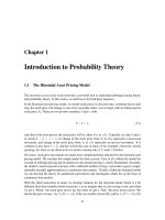
6.1 Expected Value of Discrete Random Variables
When a large collection of numbers is assembled, as in a census, we are usually
interested not in the individual numbers, but rather in certain descriptive quantities
such as the average or the median. In general, the same is true for the probability
distribution of a numerically-valued random variable. In this and in the next section,
we shall discuss two such descriptive quantities: the expected value and the variance.
Both of these quantities apply only to numerically-valued random variables, and so
we assume, in these sections, that all random variables have numerical values. To
give some intuitive justification for our definition, we consider the following game.
Average Value
A die is rolled. If an odd number turns up, we win an amount equal to this number;
if an even number turns up, we lose an amount equal to this number. For example,
if a two turns up we lose 2, and if a three comes up we win 3. We want to decide if
this is a reasonable game to play. We first try simulation. The program Die carries
out this simulation.
The program prints the frequency and the relative frequency with which each
outcome occurs. It also calculates the average winnings. We have run the program
twice. The results are shown in Table 6.1.
In the first run we have played the game 100 times. In this run our average gain
is −.57. It looks as if the game is unfavorable, and we wonder how unfavorable it
really is. To get a better idea, we have played the game 10,000 times. In this case
our average gain is −.4949.
We note that the relative frequency of each of the six possible outcomes is quite
close to the probability 1/6 for this outcome. This corresponds to our frequency
interpretation of probability. It also suggests that for very large numbers of plays,
our average gain should be
µ =1


1
6

− 2

1
6

+3

1
6

− 4

1
6

+5

1
6

− 6

1
6

225

226 CHAPTER 6. EXPECTED VALUE AND VARIANCE
n = 100 n = 10000
Winning Frequency Relative Frequency Relative
Frequency Frequency
1 17 .17 1681 .1681
-2 17 .17 1678 .1678
3 16 .16 1626 .1626
-4 18 .18 1696 .1696
5 16 .16 1686 .1686
-6 16 .16 1633 .1633
Table 6.1: Frequencies for dice game.
=
9
6
−
12
6
= −
3
6
= −.5 .
This agrees quite well with our average gain for 10,000 plays.
We note that the value we have chosen for the average gain is obtained by taking
the possible outcomes, multiplying by the probability, and adding the results. This
suggests the following definition for the expected outcome of an experiment.
Expected Value
Definition 6.1 Let X be a numerically-valued discrete random variable with sam-
ple space Ω and distribution function m(x). The expected value E(X) is defined
by
E(X)=


x∈Ω
xm(x) ,
provided this sum converges absolutely. We often refer to the expected value as
the mean, and denote E(X)byµ for short. If the above sum does not converge
absolutely, then we say that X does not have an expected value. ✷
Example 6.1 Let an experiment consist of tossing a fair coin three times. Let
X denote the number of heads which appear. Then the possible values of X are
0, 1, 2 and 3. The corresponding probabilities are 1/8, 3/8, 3/8, and 1/8. Thus, the
expected value of X equals
0

1
8

+1

3
8

+2

3
8

+3

1
8


=
3
2
.
Later in this section we shall see a quicker way to compute this expected value,
based on the fact that X can be written as a sum of simpler random variables. ✷
Example 6.2 Suppose that we toss a fair coin until a head first comes up, and let
X represent the number of tosses which were made. Then the possible values of X
are 1, 2, , and the distribution function of X is defined by
m(i)=
1
2
i
.

6.1. EXPECTED VALUE 227
(This is just the geometric distribution with parameter 1/2.) Thus, we have
E(X)=
∞

i=1
i
1
2
i
=
∞

i=1
1

2
i
+
∞

i=2
1
2
i
+ ···
=1+
1
2
+
1
2
2
+ ···
=2.
✷
Example 6.3 (Example 6.2 continued) Suppose that we flip a coin until a head
first appears, and if the number of tosses equals n, then we are paid 2
n
dollars.
What is the expected value of the payment?
We let Y represent the payment. Then,
P (Y =2
n
)=
1

2
n
,
for n ≥ 1. Thus,
E(Y )=
∞

n=1
2
n
1
2
n
,
which is a divergent sum. Thus, Y has no expectation. This example is called
the St. Petersburg Paradox . The fact that the above sum is infinite suggests that
a player should be willing to pay any fixed amount per game for the privilege of
playing this game. The reader is asked to consider how much he or she would be
willing to pay for this privilege. It is unlikely that the reader’s answer is more than
10 dollars; therein lies the paradox.
In the early history of probability, various mathematicians gave ways to resolve
this paradox. One idea (due to G. Cramer) consists of assuming that the amount
of money in the world is finite. He thus assumes that there is some fixed value of
n such that if the number of tosses equals or exceeds n, the payment is 2
n
dollars.
The reader is asked to show in Exercise 20 that the expected value of the payment
is now finite.
Daniel Bernoulli and Cramer also considered another way to assign value to
the payment. Their idea was that the value of a payment is some function of the

payment; such a function is now called a utility function. Examples of reasonable
utility functions might include the square-root function or the logarithm function.
In both cases, the value of 2n dollars is less than twice the value of n dollars. It
can easily be shown that in both cases, the expected utility of the payment is finite
(see Exercise 20). ✷

228 CHAPTER 6. EXPECTED VALUE AND VARIANCE
Example 6.4 Let T be the time for the first success in a Bernoulli trials process.
Then we take as sample space Ω the integers 1, 2, and assign the geometric
distribution
m(j)=P(T = j)=q
j−1
p.
Thus,
E(T)=1·p +2qp +3q
2
p + ···
= p(1+2q +3q
2
+ ···) .
Now if |x| < 1, then
1+x + x
2
+ x
3
+ ···=
1
1 −x
.
Differentiating this formula, we get

1+2x +3x
2
+ ···=
1
(1 −x)
2
,
so
E(T)=
p
(1 −q)
2
=
p
p
2
=
1
p
.
In particular, we see that if we toss a fair coin a sequence of times, the expected
time until the first heads is 1/(1/2) = 2. If we roll a die a sequence of times, the
expected number of rolls until the first six is 1/(1/6) = 6. ✷
Interpretation of Expected Value
In statistics, one is frequently concerned with the average value of a set of data.
The following example shows that the ideas of average value and expected value are
very closely related.
Example 6.5 The heights, in inches, of the women on the Swarthmore basketball
team are 5’ 9”, 5’ 9”, 5’ 6”, 5’ 8”, 5’ 11”, 5’ 5”, 5’ 7”, 5’ 6”, 5’ 6”, 5’ 7”, 5’ 10”, and
6’ 0”.

A statistician would compute the average height (in inches) as follows:
69+69+66+68+71+65+67+66+66+67+70+72
12
=67.9 .
One can also interpret this number as the expected value of a random variable. To
see this, let an experiment consist of choosing one of the women at random, and let
X denote her height. Then the expected value of X equals 67.9. ✷
Of course, just as with the frequency interpretation of probability, to interpret
expected value as an average outcome requires further justification. We know that
for any finite experiment the average of the outcomes is not predictable. However,
we shall eventually prove that the average will usually be close to E(X) if we repeat
the experiment a large number of times. We first need to develop some properties of
the expected value. Using these properties, and those of the concept of the variance

6.1. EXPECTED VALUE 229
XY
HHH 1
HHT 2
HTH 3
HTT 2
THH 2
THT 3
TTH 2
TTT 1
Table 6.2: Tossing a coin three times.
to be introduced in the next section, we shall be able to prove the LawofLarge
Numbers. This theorem will justify mathematically both our frequency concept
of probability and the interpretation of expected value as the average value to be
expected in a large number of experiments.
Expectation of a Function of a Random Variable

Suppose that X is a discrete random variable with sample space Ω, and φ(x)is
a real-valued function with domain Ω. Then φ(X) is a real-valued random vari-
able. One way to determine the expected value of φ(X) is to first determine the
distribution function of this random variable, and then use the definition of expec-
tation. However, there is a better way to compute the expected value of φ(X), as
demonstrated in the next example.
Example 6.6 Suppose a coin is tossed 9 times, with the result
HHHTTTTHT .
The first set of three heads is called a run. There are three more runs in this
sequence, namely the next four tails, the next head, and the next tail. We do not
consider the first two tosses to constitute a run, since the third toss has the same
value as the first two.
Now suppose an experiment consists of tossing a fair coin three times. Find the
expected number of runs. It will be helpful to think of two random variables, X
and Y , associated with this experiment. We let X denote the sequence of heads and
tails that results when the experiment is performed, and Y denote the number of
runs in the outcome X. The possible outcomes of X and the corresponding values
of Y are shown in Table 6.2.
To calculate E(Y ) using the definition of expectation, we first must find the
distribution function m(y)ofY i.e., we group together those values of X with a
common value of Y and add their probabilities. In this case, we calculate that the
distribution function of Y is: m(1)=1/4,m(2)=1/2, and m(3)=1/4. One easily
finds that E(Y )=2.

230 CHAPTER 6. EXPECTED VALUE AND VARIANCE
Now suppose we didn’t group the values of X with a common Y -value, but
instead, for each X-value x, we multiply the probability of x and the corresponding
value of Y , and add the results. We obtain
1


1
8

+2

1
8

+3

1
8

+2

1
8

+2

1
8

+3

1
8

+2


1
8

+1

1
8

,
which equals 2.
This illustrates the following general principle. If X and Y are two random
variables, and Y can be written as a function of X, then one can compute the
expected value of Y using the distribution function of X. ✷
Theorem 6.1 If X is a discrete random variable with sample space Ω and distri-
bution function m(x), and if φ :Ω→ R is a function, then
E(φ(X)) =

x∈Ω
φ(x)m(x) ,
provided the series converges absolutely. ✷
The proof of this theorem is straightforward, involving nothing more than group-
ing values of X with a common Y -value, as in Example 6.6.
The Sum of Two Random Variables
Many important results in probability theory concern sums of random variables.
We first consider what it means to add two random variables.
Example 6.7 We flip a coin and let X have the value 1 if the coin comes up heads
and 0 if the coin comes up tails. Then, we roll a die and let Y denote the face that
comes up. What does X + Y mean, and what is its distribution? This question
is easily answered in this case, by considering, as we did in Chapter 4, the joint
random variable Z =(X, Y ), whose outcomes are ordered pairs of the form (x, y),

where 0 ≤ x ≤ 1 and 1 ≤ y ≤ 6. The description of the experiment makes it
reasonable to assume that X and Y are independent, so the distribution function
of Z is uniform, with 1/12 assigned to each outcome. Now it is an easy matter to
find the set of outcomes of X + Y , and its distribution function. ✷
In Example 6.1, the random variable X denoted the number of heads which
occur when a fair coin is tossed three times. It is natural to think of X as the
sum of the random variables X
1
,X
2
,X
3
, where X
i
is defined to be 1 if the ith toss
comes up heads, and 0 if the ith toss comes up tails. The expected values of the
X
i
’s are extremely easy to compute. It turns out that the expected value of X can
be obtained by simply adding the expected values of the X
i
’s. This fact is stated
in the following theorem.

6.1. EXPECTED VALUE 231
Theorem 6.2 Let X and Y be random variables with finite expected values. Then
E(X + Y )=E(X)+E(Y ) ,
and if c is any constant, then
E(cX)=cE(X) .
Proof. Let the sample spaces of X and Y be denoted by Ω

X
and Ω
Y
, and suppose
that
Ω
X
= {x
1
,x
2
, }
and
Ω
Y
= {y
1
,y
2
, } .
Then we can consider the random variable X + Y to be the result of applying the
function φ(x, y)=x+y to the joint random variable (X, Y ). Then, by Theorem 6.1,
we have
E(X + Y )=

j

k
(x
j

+ y
k
)P (X = x
j
,Y= y
k
)
=

j

k
x
j
P (X = x
j
,Y= y
k
)+

j

k
y
k
P (X = x
j
,Y= y
k
)

=

j
x
j
P (X = x
j
)+

k
y
k
P (Y = y
k
) .
The last equality follows from the fact that

k
P (X = x
j
,Y= y
k
)=P (X = x
j
)
and

j
P (X = x
j

,Y= y
k
)=P (Y = y
k
) .
Thus,
E(X + Y )=E(X)+E(Y ) .
If c is any constant,
E(cX)=

j
cx
j
P (X = x
j
)
= c

j
x
j
P (X = x
j
)
= cE(X) .
✷

232 CHAPTER 6. EXPECTED VALUE AND VARIANCE
XY
abc 3

acb 1
bac 1
bca 0
cab 0
cba 1
Table 6.3: Number of fixed points.
It is easy to prove by mathematical induction that the expected value of the sum
of any finite number of random variables is the sum of the expected values of the
individual random variables.
It is important to note that mutual independence of the summands was not
needed as a hypothesis in the Theorem 6.2 and its generalization. The fact that
expectations add, whether or not the summands are mutually independent, is some-
times referred to as the First Fundamental Mystery of Probability.
Example 6.8 Let Y be the number of fixed points in a random permutation of
the set {a, b, c}. To find the expected value of Y , it is helpful to consider the basic
random variable associated with this experiment, namely the random variable X
which represents the random permutation. There are six possible outcomes of X,
and we assign to each of them the probability 1/6 see Table 6.3. Then we can
calculate E(Y ) using Theorem 6.1, as
3

1
6

+1

1
6

+1


1
6

+0

1
6

+0

1
6

+1

1
6

=1.
We now give a very quick way to calculate the average number of fixed points
in a random permutation of the set {1, 2, 3, ,n}. Let Z denote the random
permutation. For each i,1≤ i ≤ n, let X
i
equal 1 if Z fixes i, and 0 otherwise. So
if we let F denote the number of fixed points in Z, then
F = X
1
+ X
2

+ ···+ X
n
.
Therefore, Theorem 6.2 implies that
E(F)=E(X
1
)+E(X
2
)+···+ E(X
n
) .
But it is easy to see that for each i,
E(X
i
)=
1
n
,
so
E(F)=1.
This method of calculation of the expected value is frequently very useful. It applies
whenever the random variable in question can be written as a sum of simpler random
variables. We emphasize again that it is not necessary that the summands be
mutually independent. ✷

6.1. EXPECTED VALUE 233
Bernoulli Trials
Theorem 6.3 Let S
n
be the number of successes in n Bernoulli trials with prob-

ability p for success on each trial. Then the expected number of successes is np.
That is,
E(S
n
)=np .
Proof. Let X
j
be a random variable which has the value 1 if the jth outcome is a
success and 0 if it is a failure. Then, for each X
j
,
E(X
j
)=0· (1 − p)+1·p = p.
Since
S
n
= X
1
+ X
2
+ ···+ X
n
,
and the expected value of the sum is the sum of the expected values, we have
E(S
n
)=E(X
1
)+E(X

2
)+···+ E(X
n
)
= np .
✷
Poisson Distribution
Recall that the Poisson distribution with parameter λ was obtained as a limit of
binomial distributions with parameters n and p, where it was assumed that np = λ,
and n →∞. Since for each n, the corresponding binomial distribution has expected
value λ, it is reasonable to guess that the expected value of a Poisson distribution
with parameter λ also has expectation equal to λ. This is in fact the case, and the
reader is invited to show this (see Exercise 21).
Independence
If X and Y are two random variables, it is not true in general that E(X · Y )=
E(X)E(Y ). However, this is true if X and Y are independent.
Theorem 6.4 If X and Y are independent random variables, then
E(X ·Y )=E(X)E(Y ) .
Proof. Suppose that
Ω
X
= {x
1
,x
2
, }
and
Ω
Y
= {y

1
,y
2
, }

234 CHAPTER 6. EXPECTED VALUE AND VARIANCE
are the sample spaces of X and Y , respectively. Using Theorem 6.1, we have
E(X ·Y )=

j

k
x
j
y
k
P (X = x
j
,Y= y
k
) .
But if X and Y are independent,
P (X = x
j
,Y = y
k
)=P (X = x
j
)P (Y = y
k

) .
Thus,
E(X ·Y )=

j

k
x
j
y
k
P (X = x
j
)P (Y = y
k
)
=



j
x
j
P (X = x
j
)





k
y
k
P (Y = y
k
)

= E(X)E(Y ) .
✷
Example 6.9 A coin is tossed twice. X
i
= 1 if the ith toss is heads and 0 otherwise.
We know that X
1
and X
2
are independent. They each have expected value 1/2.
Thus E(X
1
· X
2
)=E(X
1
)E(X
2
)=(1/2)(1/2)=1/4. ✷
We next give a simple example to show that the expected values need not mul-
tiply if the random variables are not independent.
Example 6.10 Consider a single toss of a coin. We define the random variable X
to be 1 if heads turns up and 0 if tails turns up, and we set Y =1− X. Then

E(X)=E(Y )=1/2. But X · Y = 0 for either outcome. Hence, E(X · Y )=0=
E(X)E(Y ). ✷
We return to our records example of Section 3.1 for another application of the
result that the expected value of the sum of random variables is the sum of the
expected values of the individual random variables.
Records
Example 6.11 We start keeping snowfall records this year and want to find the
expected number of records that will occur in the next n years. The first year is
necessarily a record. The second year will be a record if the snowfall in the second
year is greater than that in the first year. By symmetry, this probability is 1/2.
More generally, let X
j
be1ifthejth year is a record and 0 otherwise. To find
E(X
j
), we need only find the probability that the jth year is a record. But the
record snowfall for the first j years is equally likely to fall in any one of these years,

6.1. EXPECTED VALUE 235
so E(X
j
)=1/j. Therefore, if S
n
is the total number of records observed in the
first n years,
E(S
n
)=1+
1
2

+
1
3
+ ···+
1
n
.
This is the famous divergent harmonic series. It is easy to show that
E(S
n
) ∼ log n
as n →∞.
Therefore, in ten years the expected number of records is approximately log 10 =
2.3; the exact value is the sum of the first ten terms of the harmonic series which
is 2.9. We see that, even for such a small value as n = 10, log n is not a bad
approximation. ✷
Craps
Example 6.12 In the game of craps, the player makes a bet and rolls a pair of
dice. If the sum of the numbers is 7 or 11 the player wins, if it is 2, 3, or 12 the
player loses. If any other number results, say r, then r becomes the player’s point
and he continues to roll until either r or 7 occurs. If r comes up first he wins, and
if 7 comes up first he loses. The program Craps simulates playing this game a
number of times.
We have run the program for 1000 plays in which the player bets 1 dollar each
time. The player’s average winnings were −.006. The game of craps would seem
to be only slightly unfavorable. Let us calculate the expected winnings on a single
play and see if this is the case. We construct a two-stage tree measure as shown in
Figure 6.1.
The first stage represents the possible sums for his first roll. The second stage
represents the possible outcomes for the game if it has not ended on the first roll. In

this stage we are representing the possible outcomes of a sequence of rolls required
to determine the final outcome. The branch probabilities for the first stage are
computed in the usual way assuming all 36 possibilites for outcomes for the pair of
dice are equally likely. For the second stage we assume that the game will eventually
end, and we compute the conditional probabilities for obtaining either the point or
a 7. For example, assume that the player’s point is 6. Then the game will end when
one of the eleven pairs, (1, 5), (2, 4), (3, 3), (4, 2), (5, 1), (1, 6), (2, 5), (3, 4), (4, 3),
(5, 2), (6, 1), occurs. We assume that each of these possible pairs has the same
probability. Then the player wins in the first five cases and loses in the last six.
Thus the probability of winning is 5/11 and the probability of losing is 6/11. From
the path probabilities, we can find the probability that the player wins 1 dollar; it
is 244/495. The probability of losing is then 251/495. Thus if X is his winning for
a dollar bet,
E(X)=1

244
495

+(−1)

251
495

= −
7
495
≈−.0141 .

236 CHAPTER 6. EXPECTED VALUE AND VARIANCE
W

L
W
L
W
L
W
L
W
L
W
L
(2,3,12) L
10
9
8
6
5
4
(7,11) W
1/3
2/3
2/5
3/5
5/11
6/11
5/11
6/11
2/5
3/5
1/3

2/3
2/9
1/12
1/9
5/36
5/36
1/9
1/12
1/9
1/36
2/36
2/45
3/45
25/396
30/396
25/396
30/396
2/45
3/45
1/36
2/36
Figure 6.1: Tree measure for craps.

6.1. EXPECTED VALUE 237
The game is unfavorable, but only slightly. The player’s expected gain in n plays is
−n(.0141). If n is not large, this is a small expected loss for the player. The casino
makes a large number of plays and so can afford a small average gain per play and
still expect a large profit. ✷
Roulette
Example 6.13 In Las Vegas, a roulette wheel has 38 slots numbered 0, 00, 1, 2,

, 36. The 0 and 00 slots are green, and half of the remaining 36 slots are red
and half are black. A croupier spins the wheel and throws an ivory ball. If you bet
1 dollar on red, you win 1 dollar if the ball stops in a red slot, and otherwise you
lose a dollar. We wish to calculate the expected value of your winnings, if you bet
1 dollar on red.
Let X be the random variable which denotes your winnings in a 1 dollar bet on
red in Las Vegas roulette. Then the distribution of X is given by
m
X
=

−11
20/38 18/38

,
and one can easily calculate (see Exercise 5) that
E(X) ≈−.0526 .
We now consider the roulette game in Monte Carlo, and follow the treatment
of Sagan.
1
In the roulette game in Monte Carlo there is only one 0. If you bet 1
franc on red and a 0 turns up, then, depending upon the casino, one or more of the
following options may be offered:
(a) You get 1/2 of your bet back, and the casino gets the other half of your bet.
(b) Your bet is put “in prison,” which we will denote by P
1
. If red comes up on
the next turn, you get your bet back (but you don’t win any money). If black or 0
comes up, you lose your bet.
(c) Your bet is put in prison P

1
, as before. If red comes up on the next turn, you
get your bet back, and if black comes up on the next turn, then you lose your bet.
If a 0 comes up on the next turn, then your bet is put into double prison, which we
will denote by P
2
. If your bet is in double prison, and if red comes up on the next
turn, then your bet is moved back to prison P
1
and the game proceeds as before.
If your bet is in double prison, and if black or 0 come up on the next turn, then
you lose your bet. We refer the reader to Figure 6.2, where a tree for this option is
shown. In this figure, S is the starting position, W means that you win your bet,
L means that you lose your bet, and E means that you break even.
It is interesting to compare the expected winnings of a 1 franc bet on red, under
each of these three options. We leave the first two calculations as an exercise (see
Exercise 37). Suppose that you choose to play alternative (c). The calculation for
this case illustrates the way that the early French probabilists worked problems like
this.
1
H. Sagan, Markov Chains in Monte Carlo, Math. Mag., vol. 54, no. 1 (1981), pp. 3-10.

238 CHAPTER 6. EXPECTED VALUE AND VARIANCE
S
W
L
E
L
L
L

L
L
L
E
P
1
P
1
P
1
P
2
P
2
P
2
Figure 6.2: Tree for 2-prison Monte Carlo roulette.
Suppose you bet on red, you choose alternative (c), and a 0 comes up. Your
possible future outcomes are shown in the tree diagram in Figure 6.3. Assume that
your money is in the first prison and let x be the probability that you lose your
franc. From the tree diagram we see that
x =
18
37
+
1
37
P (you lose your franc | your franc is in P
2
) .

Also,
P (you lose your franc | your franc is in P
2
)=
19
37
+
18
37
x.
So, we have
x =
18
37
+
1
37

19
37
+
18
37
x

.
Solving for x, we obtain x = 685/1351. Thus, starting at S, the probability that
you lose your bet equals
18
37

+
1
37
x =
25003
49987
.
To find the probability that you win when you bet on red, note that you can
only win if red comes up on the first turn, and this happens with probability 18/37.
Thus your expected winnings are
1 ·
18
37
− 1 ·
25003
49987
= −
687
49987
≈−.0137 .
It is interesting to note that the more romantic option (c) is less favorable than
option (a) (see Exercise 37).

6.1. EXPECTED VALUE 239
PW
L
P
P
L
18/37

18/37
1/37
19/37
18/37
1
1
2
Figure 6.3: Your money is put in prison.
If you bet 1 dollar on the number 17, then the distribution function for your
winnings X is
P
X
=

−135
36/37 1/37

,
and the expected winnings are
−1 ·
36
37
+35·
1
37
= −
1
37
≈−.027 .
Thus, at Monte Carlo different bets have different expected values. In Las Vegas

almost all bets have the same expected value of −2/38 = −.0526 (see Exercises 4
and 5). ✷
Conditional Expectation
Definition 6.2 If F is any event and X is a random variable with sample space
Ω={x
1
,x
2
, }, then the conditional expectation given F is defined by
E(X|F)=

j
x
j
P (X = x
j
|F ) .
Conditional expectation is used most often in the form provided by the following
theorem. ✷
Theorem 6.5 Let X be a random variable with sample space Ω. If F
1
, F
2
, ,F
r
are events such that F
i
∩ F
j
= ∅ for i = j and Ω = ∪

j
F
j
, then
E(X)=

j
E(X|F
j
)P (F
j
) .

240 CHAPTER 6. EXPECTED VALUE AND VARIANCE
Proof. We have

j
E(X|F
j
)P (F
j
)=

j

k
x
k
P (X = x
k

|F
j
)P (F
j
)
=

j

k
x
k
P (X = x
k
and F
j
occurs)
=

k

j
x
k
P (X = x
k
and F
j
occurs)
=


k
x
k
P (X = x
k
)
= E(X) .
✷
Example 6.14 (Example 6.12 continued) Let T be the number of rolls in a single
play of craps. We can think of a single play as a two-stage process. The first stage
consists of a single roll of a pair of dice. The play is over if this roll is a 2, 3, 7,
11, or 12. Otherwise, the player’s point is established, and the second stage begins.
This second stage consists of a sequence of rolls which ends when either the player’s
pointora7isrolled. We record the outcomes of this two-stage experiment using
the random variables X and S, where X denotes the first roll, and S denotes the
number of rolls in the second stage of the experiment (of course, S is sometimes
equal to 0). Note that T = S + 1. Then by Theorem 6.5
E(T)=
12

j=2
E(T|X = j)P(X = j) .
If j = 7, 11 or 2, 3, 12, then E(T |X = j)=1. Ifj =4, 5, 6, 8, 9, or 10, we can
use Example 6.4 to calculate the expected value of S. In each of these cases, we
continue rolling until we get either a j or a 7. Thus, S is geometrically distributed
with parameter p, which depends upon j.Ifj = 4, for example, the value of p is
3/36+6/36=1/4. Thus, in this case, the expected number of additional rolls is
1/p =4,soE(T |X = 4) = 1 + 4 = 5. Carrying out the corresponding calculations
for the other possible values of j and using Theorem 6.5 gives

E(T)=1

12
36

+

1+
36
3+6

3
36

+

1+
36
4+6

4
36

+

1+
36
5+6

5

36

+

1+
36
5+6

5
36

+

1+
36
4+6

4
36

+

1+
36
3+6

3
36

=

557
165
≈ 3.375 .
✷

6.1. EXPECTED VALUE 241
Martingales
We can extend the notion of fairness to a player playing a sequence of games by
using the concept of conditional expectation.
Example 6.15 Let S
1
, S
2
, ,S
n
be Peter’s accumulated fortune in playing heads
or tails (see Example 1.4). Then
E(S
n
|S
n−1
= a, ,S
1
= r)=
1
2
(a +1)+
1
2
(a −1) = a.

We note that Peter’s expected fortune after the next play is equal to his present
fortune. When this occurs, we say the game is fair. A fair game is also called a
martingale. If the coin is biased and comes up heads with probability p and tails
with probability q =1− p, then
E(S
n
|S
n−1
= a, ,S
1
= r)=p(a +1)+q(a − 1) = a + p − q.
Thus, if p<q, this game is unfavorable, and if p>q, it is favorable. ✷
If you are in a casino, you will see players adopting elaborate systems of play
to try to make unfavorable games favorable. Two such systems, the martingale
doubling system and the more conservative Labouchere system, were described in
Exercises 1.1.9 and 1.1.10. Unfortunately, such systems cannot change even a fair
game into a favorable game.
Even so, it is a favorite pastime of many people to develop systems of play for
gambling games and for other games such as the stock market. We close this section
with a simple illustration of such a system.
Stock Prices
Example 6.16 Let us assume that a stock increases or decreases in value each
day by 1 dollar, each with probability 1/2. Then we can identify this simplified
model with our familiar game of heads or tails. We assume that a buyer, Mr. Ace,
adopts the following strategy. He buys the stock on the first day at its price V .
He then waits until the price of the stock increases by one to V + 1 and sells. He
then continues to watch the stock until its price falls back to V . He buys again and
waits until it goes up to V + 1 and sells. Thus he holds the stock in intervals during
which it increases by 1 dollar. In each such interval, he makes a profit of 1 dollar.
However, we assume that he can do this only for a finite number of trading days.

Thus he can lose if, in the last interval that he holds the stock, it does not get
backuptoV + 1; and this is the only we he can lose. In Figure 6.4 we illustrate a
typical history if Mr. Ace must stop in twenty days. Mr. Ace holds the stock under
his system during the days indicated by broken lines. We note that for the history
shown in Figure 6.4, his system nets him a gain of 4 dollars.
We have written a program StockSystem to simulate the fortune of Mr. Ace
if he uses his sytem over an n-day period. If one runs this program a large number

242 CHAPTER 6. EXPECTED VALUE AND VARIANCE
5 10 15 20
-1
-0.5
0.5
1
1.5
2
Figure 6.4: Mr. Ace’s system.
of times, for n = 20, say, one finds that his expected winnings are very close to 0,
but the probability that he is ahead after 20 days is significantly greater than 1/2.
For small values of n, the exact distribution of winnings can be calculated. The
distribution for the case n = 20 is shown in Figure 6.5. Using this distribution,
it is easy to calculate that the expected value of his winnings is exactly 0. This
is another instance of the fact that a fair game (a martingale) remains fair under
quite general systems of play.
Although the expected value of his winnings is 0, the probability that Mr. Ace is
ahead after 20 days is about .610. Thus, he would be able to tell his friends that his
system gives him a better chance of being ahead than that of someone who simply
buys the stock and holds it, if our simple random model is correct. There have been
a number of studies to determine how random the stock market is. ✷
Historical Remarks

With the Law of Large Numbers to bolster the frequency interpretation of proba-
bility, we find it natural to justify the definition of expected value in terms of the
average outcome over a large number of repetitions of the experiment. The concept
of expected value was used before it was formally defined; and when it was used,
it was considered not as an average value but rather as the appropriate value for a
gamble. For example, recall Pascal’s way of finding the value of a three-game series
that had to be called off before it is finished.
Pascal first observed that if each player has only one game to win, then the
stake of 64 pistoles should be divided evenly. Then he considered the case where
one player has won two games and the other one.
Then consider, Sir, if the first man wins, he gets 64 pistoles, if he loses
he gets 32. Thus if they do not wish to risk this last game, but wish
to separate without playing it, the first man must say: “I am certain

6.1. EXPECTED VALUE 243
-20 -15 -10 -5 0 5 10
0
0.05
0.1
0.15
0.2
Figure 6.5: Winnings distribution for n = 20.
to get 32 pistoles, even if I lose I still get them; but as for the other
32 pistoles, perhaps I will get them, perhaps you will get them, the
chances are equal. Let us then divide these 32 pistoles in half and give
one half to me as well as my 32 which are mine for sure.” He will then
have 48 pistoles and the other 16.
2
Note that Pascal reduced the problem to a symmetric bet in which each player
gets the same amount and takes it as obvious that in this case the stakes should be

divided equally.
The first systematic study of expected value appears in Huygens’ book. Like
Pascal, Huygens find the value of a gamble by assuming that the answer is obvious
for certain symmetric situations and uses this to deduce the expected for the general
situation. He does this in steps. His first proposition is
Prop. I. If I expect a or b, either of which, with equal probability, may
fall to me, then my Expectation is worth (a+b)/2, that is, the half Sum
of a and b.
3
Huygens proved this as follows: Assume that two player A and B play a game in
which each player puts up a stake of (a + b)/2 with an equal chance of winning the
total stake. Then the value of the game to each player is (a + b)/2. For example, if
the game had to be called off clearly each player should just get back his original
stake. Now, by symmetry, this value is not changed if we add the condition that
the winner of the game has to pay the loser an amount b as a consolation prize.
Then for player A the value is still (a + b)/2. But what are his possible outcomes
for the modified game? If he wins he gets the total stake a + b and must pay B an
2
Quoted in F. N. David, Games, Gods and Gambling (London: Griffin, 1962), p. 231.
3
C. Huygens, Calculating in Games of Chance, translation attributed to John Arbuthnot (Lon-
don, 1692), p. 34.

244 CHAPTER 6. EXPECTED VALUE AND VARIANCE
amount b so ends up with a. If he loses he gets an amount b from player B. Thus
player A wins a or b with equal chances and the value to him is (a + b)/2.
Huygens illustrated this proof in terms of an example. If you are offered a game
in which you have an equal chance of winning 2 or 8, the expected value is 5, since
this game is equivalent to the game in which each player stakes 5 and agrees to pay
the loser3—agame in which the value is obviously 5.

Huygens’ second proposition is
Prop. II. If I expect a, b,orc, either of which, with equal facility, may
happen, then the Value of my Expectation is (a + b + c)/3, or the third
of the Sum of a, b, and c.
4
His argument here is similar. Three players, A, B, and C, each stake
(a + b + c)/3
in a game they have an equal chance of winning. The value of this game to player
A is clearly the amount he has staked. Further, this value is not changed if A enters
into an agreement with B that if one of them wins he pays the other a consolation
prize of b and with C that if one of them wins he pays the other a consolation prize
of c. By symmetry these agreements do not change the value of the game. In this
modified game, if A wins he wins the total stake a + b + c minus the consolation
prizes b + c giving him a final winning of a. If B wins, A wins b and if C wins, A
wins c. Thus A finds himself in a game with value (a + b + c)/3 and with outcomes
a, b, and c occurring with equal chance. This proves Proposition II.
More generally, this reasoning shows that if there are n outcomes
a
1
,a
2
, , a
n
,
all occurring with the same probability, the expected value is
a
1
+ a
2
+ ···+ a

n
n
.
In his third proposition Huygens considered the case where you win a or b but
with unequal probabilities. He assumed there are p chances of winning a, and q
chances of winning b, all having the same probability. He then showed that the
expected value is
E =
p
p + q
· a +
q
p + q
· b.
This follows by considering an equivalent gamble with p + q outcomes all occurring
with the same probability and with a payoff of a in p of the outcomes and b in q of
the outcomes. This allowed Huygens to compute the expected value for experiments
with unequal probabilities, at least when these probablities are rational numbers.
Thus, instead of defining the expected value as a weighted average, Huygens
assumed that the expected value of certain symmetric gambles are known and de-
duced the other values from these. Although this requires a good deal of clever
4
ibid., p. 35.

6.1. EXPECTED VALUE 245
manipulation, Huygens ended up with values that agree with those given by our
modern definition of expected value. One advantage of this method is that it gives
a justification for the expected value in cases where it is not reasonable to assume
that you can repeat the experiment a large number of times, as for example, in
betting that at least two presidents died on the same day of the year. (In fact,

three did; all were signers of the Declaration of Independence, and all three died on
July 4.)
In his book, Huygens calculated the expected value of games using techniques
similar to those which we used in computing the expected value for roulette at
Monte Carlo. For example, his proposition XIV is:
Prop. XIV. If I were playing with another by turns, with two Dice, on
this Condition, that if I throw 7 I gain, and if he throws 6 he gains
allowing him the first Throw: To find the proportion of my Hazard to
his.
5
A modern description of this game is as follows. Huygens and his opponent take
turns rolling a die. The game is over if Huygens rollsa7orhisopponent rolls a 6.
His opponent rolls first. What is the probability that Huygens wins the game?
To solve this problem Huygens let x be his chance of winning when his opponent
threw first and y his chance of winning when he threw first. Then on the first roll
his opponent wins on 5 out of the 36 possibilities. Thus,
x =
31
36
· y.
But when Huygens rolls he wins on 6 out of the 36 possible outcomes, and in the
other 30, he is led back to where his chances are x.Thus
y =
6
36
+
30
36
· x.
From these two equations Huygens found that x =31/61.

Another early use of expected value appeared in Pascal’s argument to show that
a rational person should believe in the existence of God.
6
Pascal said that we have
to make a wager whether to believe or not to believe. Let p denote the probability
that God does not exist. His discussion suggests that we are playing a game with
two strategies, believe and not believe, with payoffs as shown in Table 6.4.
Here −u represents the cost to you of passing up some worldly pleasures as
a consequence of believing that God exists. If you do not believe, and God is a
vengeful God, you will lose x. If God exists and you do believe you will gain v.
Now to determine which strategy is best you should compare the two expected
values
p(−u)+(1− p)v and p0+(1− p)(−x),
5
ibid., p. 47.
6
Quoted in I. Hacking, The Emergence of Probability (Cambridge: Cambridge Univ. Press,
1975).

246 CHAPTER 6. EXPECTED VALUE AND VARIANCE
God does not exist God exists
p 1 −p
believe −u v
not believe 0 −x
Table 6.4: Payoffs.
Age Survivors
0 100
664
16 40
26 25

36 16
46 10
56 6
66 3
76 1
Table 6.5: Graunt’s mortality data.
and choose the larger of the two. In general, the choice will depend upon the value of
p. But Pascal assumed that the value of v is infinite and so the strategy of believing
is best no matter what probability you assign for the existence of God. This example
is considered by some to be the beginning of decision theory. Decision analyses of
this kind appear today in many fields, and, in particular, are an important part of
medical diagnostics and corporate business decisions.
Another early use of expected value was to decide the price of annuities. The
study of statistics has its origins in the use of the bills of mortality kept in the
parishes in London from 1603. These records kept a weekly tally of christenings
and burials. From these John Graunt made estimates for the population of London
and also provided the first mortality data,
7
shown in Table 6.5.
As Hacking observes, Graunt apparently constructed this table by assuming
that after the age of 6 there is a constant probability of about 5/8 of surviving
for another decade.
8
For example, of the 64 people who survive to age 6, 5/8 of
64 or 40 survive to 16, 5/8 of these 40 or 25 survive to 26, and so forth. Of course,
he rounded off his figures to the nearest whole person.
Clearly, a constant mortality rate cannot be correct throughout the whole range,
and later tables provided by Halley were more realistic in this respect.
9
7

ibid., p. 108.
8
ibid., p. 109.
9
E. Halley, “An Estimate of The Degrees of Mortality of Mankind,” Phil. Trans. Royal. Soc.,

6.1. EXPECTED VALUE 247
A terminal annuity provides a fixed amount of money during a period of n years.
To determine the price of a terminal annuity one needs only to know the appropriate
interest rate. A life annuity provides a fixed amount during each year of the buyer’s
life. The appropriate price for a life annuity is the expected value of the terminal
annuity evaluated for the random lifetime of the buyer. Thus, the work of Huygens
in introducing expected value and the work of Graunt and Halley in determining
mortality tables led to a more rational method for pricing annuities. This was one
of the first serious uses of probability theory outside the gambling houses.
Although expected value plays a role now in every branch of science, it retains
its importance in the casino. In 1962, Edward Thorp’s book Beat the Dealer
10
provided the reader with a strategy for playing the popular casino game of blackjack
that would assure the player a positive expected winning. This book forevermore
changed the belief of the casinos that they could not be beat.
Exercises
1 A card is drawn at random from a deck consisting of cards numbered 2
through 10. A player wins 1 dollar if the number on the card is odd and
loses 1 dollar if the number if even. What is the expected value of his win-
nings?
2 A card is drawn at random from a deck of playing cards. If it is red, the player
wins 1 dollar; if it is black, the player loses 2 dollars. Find the expected value
of the game.
3 In a class there are 20 students: 3 are 5’ 6”, 5 are 5’8”, 4 are 5’10”, 4 are

6’, and 4 are 6’ 2”. A student is chosen at random. What is the student’s
expected height?
4 In Las Vegas the roulette wheel has a 0 and a 00 and then the numbers 1 to 36
marked on equal slots; the wheel is spun and a ball stops randomly in one
slot. When a player bets 1 dollar on a number, he receives 36 dollars if the
ball stops on this number, for a net gain of 35 dollars; otherwise, he loses his
dollar bet. Find the expected value for his winnings.
5 In a second version of roulette in Las Vegas, a player bets on red or black.
Half of the numbers from 1 to 36 are red, and half are black. If a player bets
a dollar on black, and if the ball stops on a black number, he gets his dollar
back and another dollar. If the ball stops on a red number or on 0 or 00 he
loses his dollar. Find the expected winnings for this bet.
6 A die is rolled twice. Let X denote the sum of the two numbers that turn up,
and Y the difference of the numbers (specifically, the number on the first roll
minus the number on the second). Show that E(XY )=E(X)E(Y ). Are X
and Y independent?
vol. 17 (1693), pp. 596–610; 654–656.
10
E. Thorp, Beat the Dealer (New York: Random House, 1962).

248 CHAPTER 6. EXPECTED VALUE AND VARIANCE
*7 Show that, if X and Y are random variables taking on only two values each,
and if E(XY )=E(X)E(Y ), then X and Y are independent.
8 A royal family has children until it has a boy or until it has three children,
whichever comes first. Assume that each child is a boy with probability 1/2.
Find the expected number of boys in this royal family and the expected num-
ber of girls.
9 If the first roll in a game of craps is neither a natural nor craps, the player
can make an additional bet, equal to his original one, that he will make his
point before a seven turns up. If his point is four or ten he is paid off at 2 : 1

odds; if it is a five or nine he is paid off at odds 3 : 2; and if it is a six or eight
he is paid off at odds 6 : 5. Find the player’s expected winnings if he makes
this additional bet when he has the opportunity.
10 In Example 6.16 assume that Mr. Ace decides to buy the stock and hold it
until it goes up 1 dollar and then sell and not buy again. Modify the program
StockSystem to find the distribution of his profit under this system after
a twenty-day period. Find the expected profit and the probability that he
comes out ahead.
11 On September 26, 1980, the New York Times reported that a mysterious
stranger strode into a Las Vegas casino, placed a single bet of 777,000 dollars
on the “don’t pass” line at the crap table, and walked away with more than
1.5 million dollars. In the “don’t pass” bet, the bettor is essentially betting
with the house. An exception occurs if the roller rolls a 12 on the first roll.
In this case, the roller loses and the “don’t pass” better just gets back the
money bet instead of winning. Show that the “don’t pass” bettor has a more
favorable bet than the roller.
12 Recall that in the martingale doubling system (see Exercise 1.1.10), the player
doubles his bet each time he loses and quits the first time he is ahead. Suppose
that you are playing roulette in a fair casino where there are no 0’s, and you
bet on red each time. You then win with probability 1/2 each time. Assume
that you start with a 1-dollar bet and employ the martingale system. Since
you entered the casino with 100 dollars, you also quit in the unlikely event
that black turns up six times in a row so that you are down 63 dollars and
cannot make the required 64-dollar bet. Find your expected winnings under
this system of play.
13 You have 80 dollars and play the following game. An urn contains two white
balls and two black balls. You draw the balls out one at a time without
replacement until all the balls are gone. On each draw, you bet half of your
present fortune that you will draw a white ball. What is your final fortune?
14 In the hat check problem (see Example 3.12), it was assumed that N people

check their hats and the hats are handed back at random. Let X
j
= 1 if the

6.1. EXPECTED VALUE 249
jth person gets his or her hat and 0 otherwise. Find E(X
j
) and E(X
j
· X
k
)
for j not equal to k. Are X
j
and X
k
independent?
15 A box contains two gold balls and three silver balls. You are allowed to choose
successively balls from the box at random. You win 1 dollar each time you
draw a gold ball and lose 1 dollar each time you draw a silver ball. After a
draw, the ball is not replaced. Show that, if you draw until you are ahead by
1 dollar or until there are no more gold balls, this is a favorable game.
16 Gerolamo Cardano in his book, The Gambling Scholar, written in the early
1500s, considers the following carnival game. There are six dice. Each of the
dice has five blank sides. The sixth side has a number between 1 and 6—a
different number on each die. The six dice are rolled and the player wins a
prize depending on the total of the numbers which turn up.
(a) Find, as Cardano did, the expected total without finding its distribution.
(b) Large prizes were given for large totals with a modest fee to play the
game. Explain why this could be done.

17 Let X be the first time that a failure occurs in an infinite sequence of Bernoulli
trials with probability p for success. Let p
k
= P (X = k) for k = 1, 2,
Show that p
k
= p
k−1
q where q =1− p. Show that

k
p
k
= 1. Show that
E(X)=1/q. What is the expected number of tosses of a coin required to
obtain the first tail?
18 Exactly one of six similar keys opens a certain door. If you try the keys, one
after another, what is the expected number of keys that you will have to try
before success?
19 A multiple choice exam is given. A problem has four possible answers, and
exactly one answer is correct. The student is allowed to choose a subset of
the four possible answers as his answer. If his chosen subset contains the
correct answer, the student receives three points, but he loses one point for
each wrong answer in his chosen subset. Show that if he just guesses a subset
uniformly and randomly his expected score is zero.
20 You are offered the following game to play: a fair coin is tossed until heads
turns up for the first time (see Example 6.3). If this occurs on the first toss
you receive 2 dollars, if it occurs on the second toss you receive 2
2
= 4 dollars

and, in general, if heads turns up for the first time on the nth toss you receive
2
n
dollars.
(a) Show that the expected value of your winnings does not exist (i.e., is
given by a divergent sum) for this game. Does this mean that this game
is favorable no matter how much you pay to play it?
(b) Assume that you only receive 2
10
dollars if any number greater than or
equal to ten tosses are required to obtain the first head. Show that your
expected value for this modified game is finite and find its value.